Join our inaugural Reading Group in San Francisco on April 29. Register now
Out of distribution blindness: why to fix it and how energy can help
Sharon Li is an assistant professor at the University of Wisconsin-Madison. She presented “Detecting Data Distributional Shift: Challenges and Opportunities” at Snorkel AI’s The Future of Data-Centric AI Summit in 2022. The talk covered a novel approach for handling out-of-distribution objects. A transcript of her talk follows. It has been lightly edited for reading clarity.
Today I will be sharing with you some interesting challenges and opportunities around detecting data distributional shift. Hopefully, this talk will inspire you to think about, or even pursue, some of these problems in the future.
I would like to start the talk by showing you this video.
This is a model trained on the Berkeley Deep Drive-100k dataset, performing bounding box tracking on the road. Whenever we see videos like this, we may get this overly positive impression of how remarkable deep learning models are, which is true in some cases. In my research, I encourage researchers and practitioners to look at the other side as well, and especially to be aware of unexpected situations that the model wasn’t trained for.
To see what I mean, let’s think about how you would build and deploy a self-driving car model.
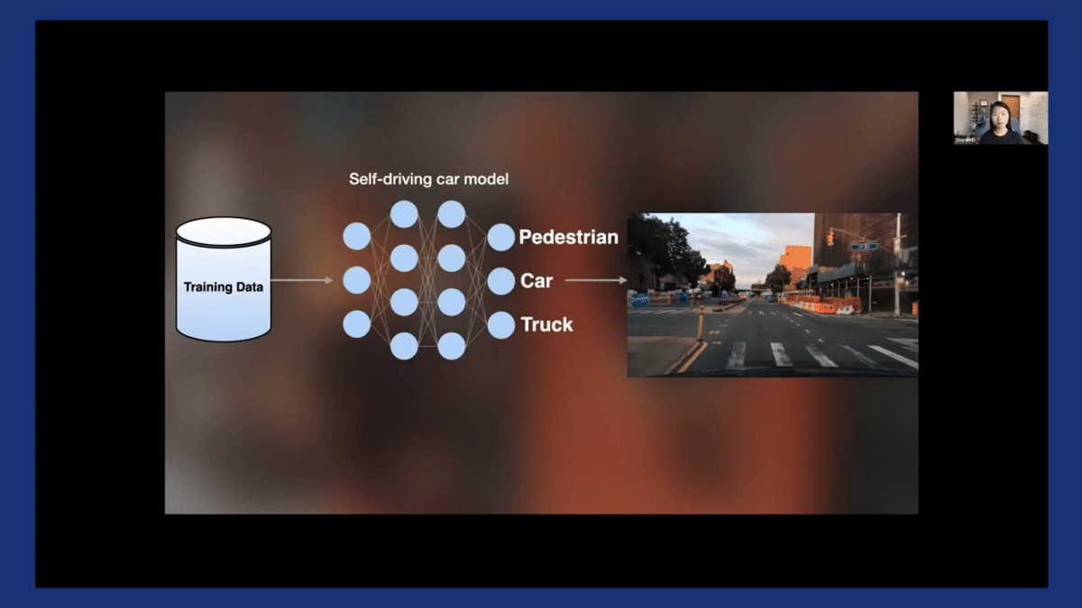
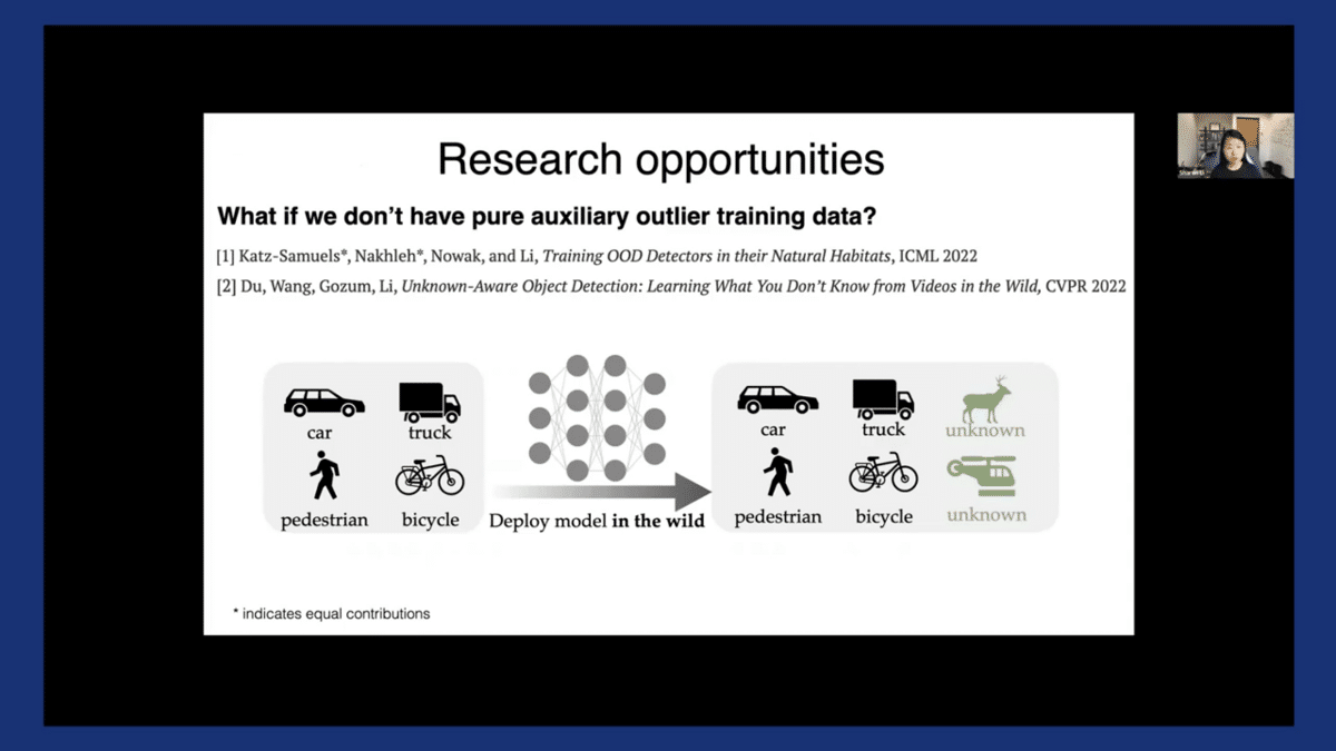
The typical process is to collect some training data with corresponding labels, and then train on your favorite machine learning model. Here, the output typically contains some predefined categories such as pedestrians and cars and trucks, and so on.
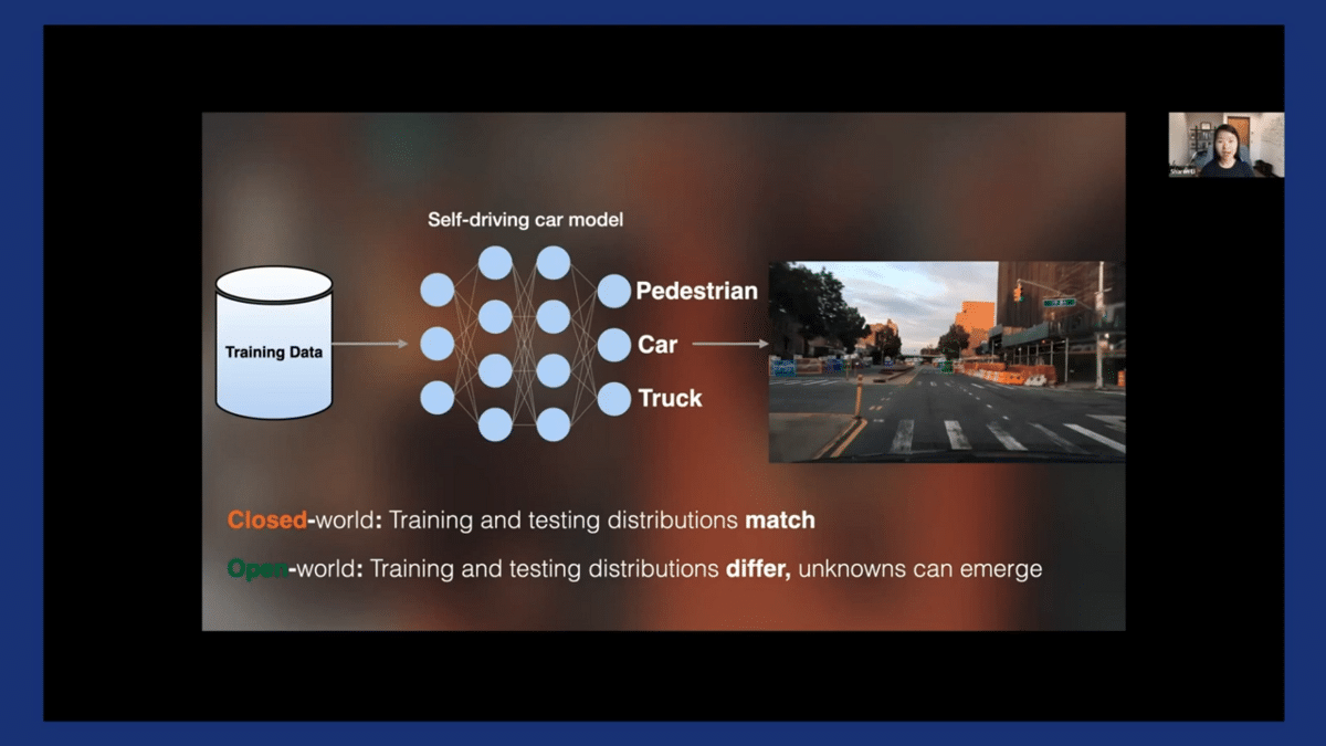
The model finally gets deployed in the wild, which is often a highly dynamic and uncertain environment. The model will inevitably encounter some new contexts and data that were not taught to this learning algorithm in training time.
This is called the open-world setting, in contrast to classic closed-world machine learning.
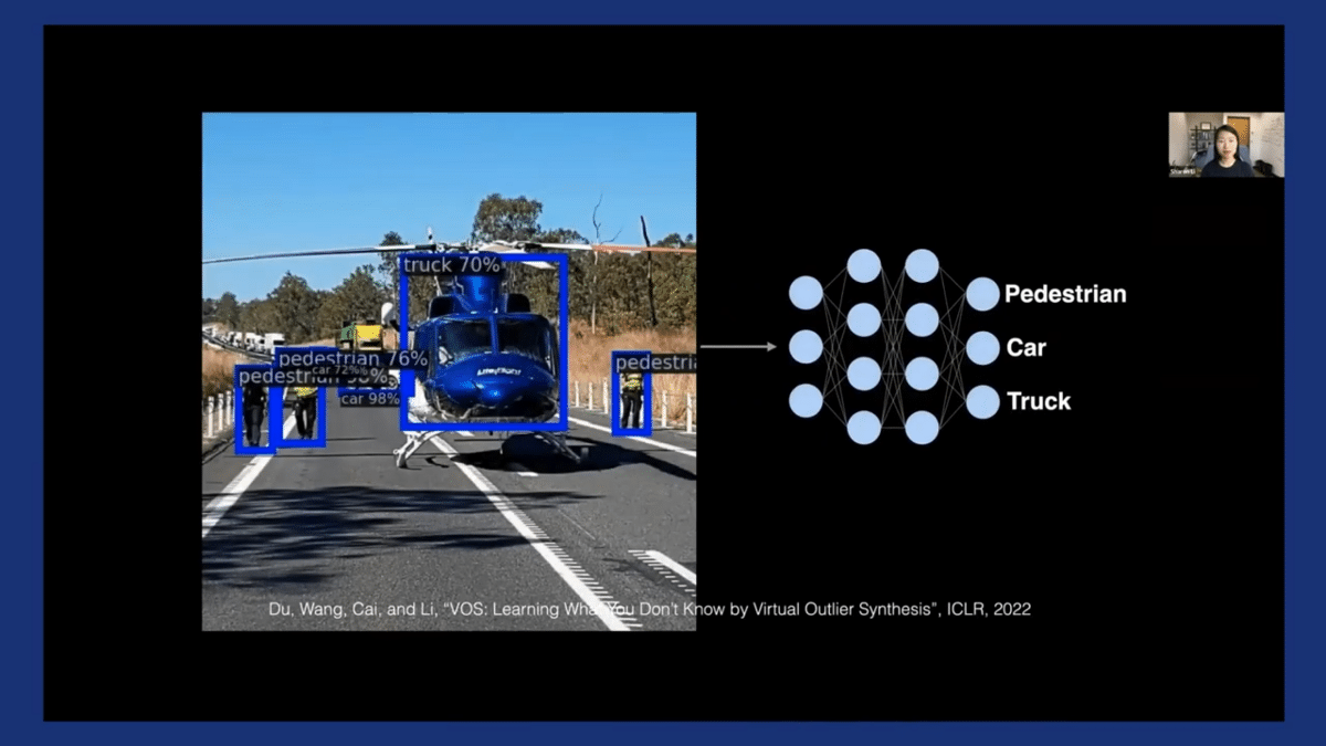
For example in our recent paper, we took this image from the MS COCO dataset and ran through the self-driving car model that was just trained on BDD. The model can produce overconfident predictions for this unknown object, the helicopter—which was never exposed to this model during its training time. It’s being predicted into a truck, which is one of the in-distribution categories. In other words, deep networks do not necessarily know what they don’t know. This has raised significant concerns about models’ reliability and safety.
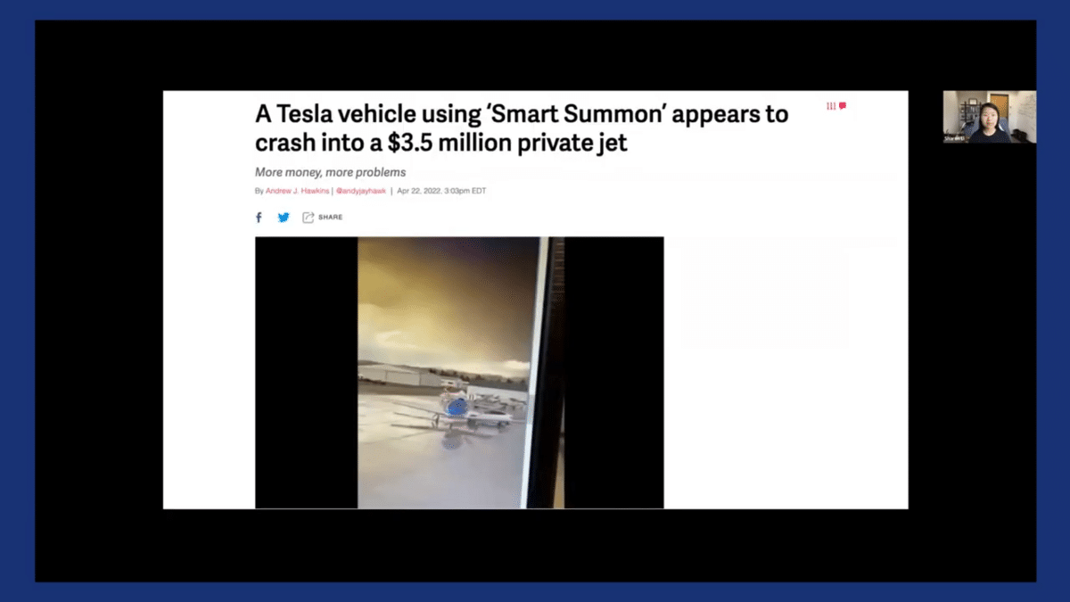
Believe it or not, this kind of event can happen in real life as well, causing huge consequences. For example, I’m quoting a news article from just about three months ago, where a Tesla vehicle was reported to crash into a private jet that’s worth $3.5 million.
This out-of-distribution detection problem has become very important. A fun story that I want to share—I remember back in 2016-2017ish when we started working on this problem and submitted one of our first papers on OOD detection called Odin to the conference. We were troubled by people questioning, “Why should we care, and why bother solving this problem?”
Fast forward six years—nowadays, if you write a paper about out-of-distribution, the first thing that the reviewer would say is, “This paper tackles a very important problem in machine learning.” It’s really great to see this increasing awareness from the research community and industry as well over time.
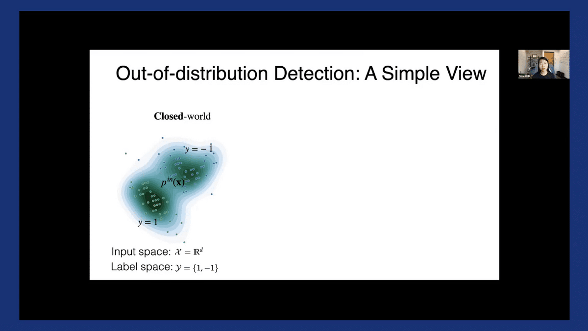
So now let’s look at this problem more formally to set up the stage. Here, let’s say we have our training data distribution, that is, a mixture of two Gaussians for class label y = {1, -1}. Our in-distribution pin would be the marginal of this joint distribution over the input space.
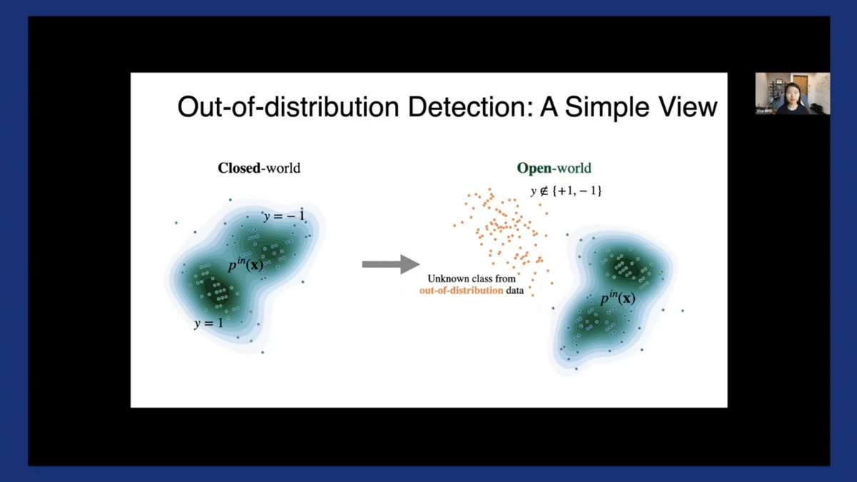
During test time, these orange dots could emerge which are out-of-distribution from an unknown class—that is, doesn’t belong to either y = 1 or y = -1 and therefore should not be predicted into these two labels.
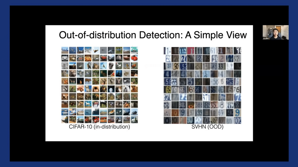
To translate this toy data into high-dimensional images, for example, you can think of CIFAR-10 on the left-hand side being the in-distribution set, and Street View House Number (or SVHN) on the right-hand side, being the OOD, which has disjoint labels.
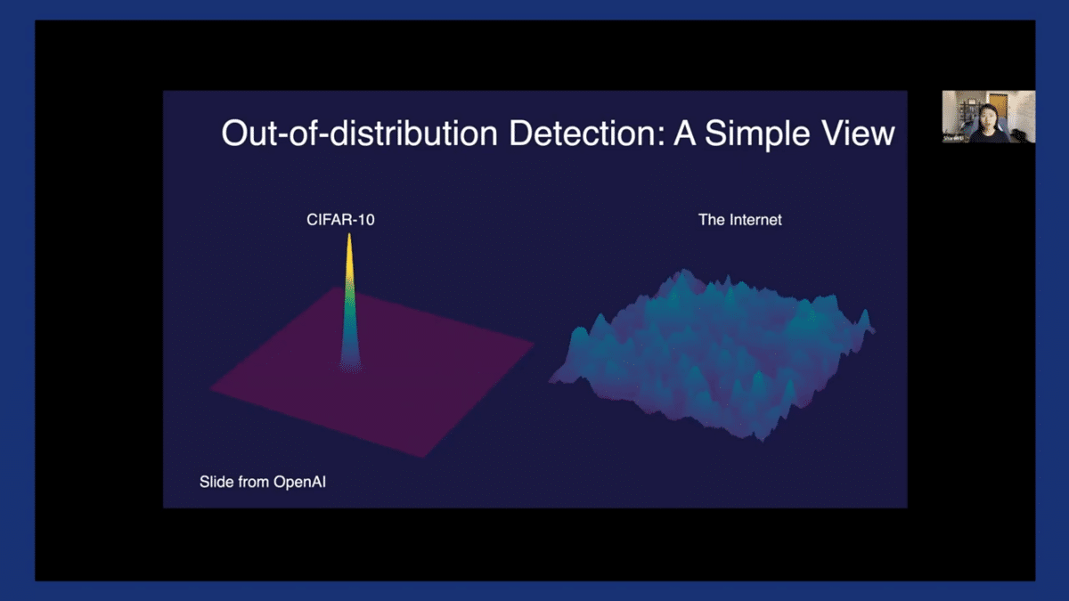
SVHN is just one of the OOD datasets that a model may encounter—there are many other unknowns on this complex data manifold. For example, as shown on the right-hand side, imagine that’s the manifold of all the possible images one could possibly generate and encounter on the internet. It’s a lot more complex compared to this task-specific dataset on the left-hand side. This image, which credits to OpenAI, really nicely illustrates the complexity of the problem.
Out-of-distribution detection is a hard problem. Before we get into the methodology, I wanted to spend a couple of slides explaining “the why”.
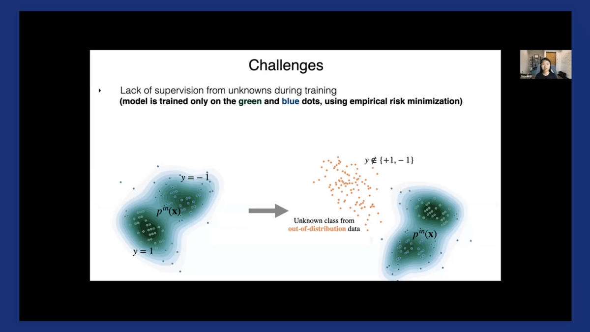
The first challenge is the lack of unknowns during training time. The model is typically trained only on the in-distribution data—in this case, the green and blue dots using empirical risk minimization. It can be difficult to anticipate where these orange dots could emerge in advance because there can be a huge space of unknowns, especially if you extrapolate those to be the high dimensional space.
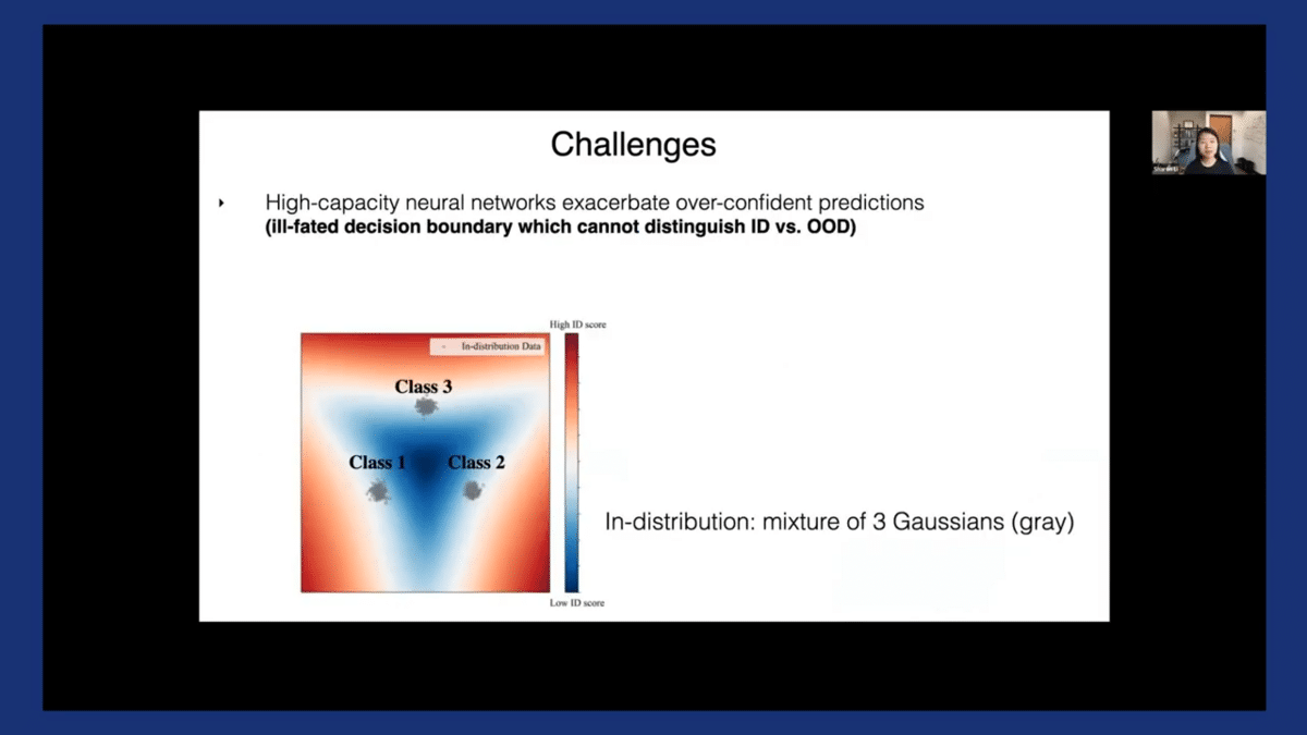
The problem is further exacerbated by the high-capacity neural networks that we are working with nowadays (that just keep getting bigger and more complex). Here, I’m showing you one of my favorite figures. This is an in-distribution classification with three classes. We have a mixture of three Gaussians highlighted in gray, and the model is trained using the standard cross-entropy laws to classify these three classes. The model learns this triangular-shaped decision boundary, which does a perfect job in terms of separating among these three classes.
However, the trouble arises when it comes to OOD detection because you see that the decision boundary is quite ill-fated. Those red regions correspond to high-confidence regions, despite being very far away from our in-distribution data. Therefore, this is a case where a model is perfectly fine for classification, but it cannot reliably tell apart ID vs. OOD.
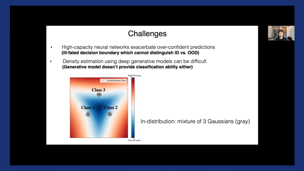
Just in case you’re wondering if we can perform density estimation to directly estimate the likelihood—it turns out, there are some challenges too. For example, training deep generative models can be hard to optimize. Moreover, generative models don’t provide classification-ability either, which is something we’re interested in.
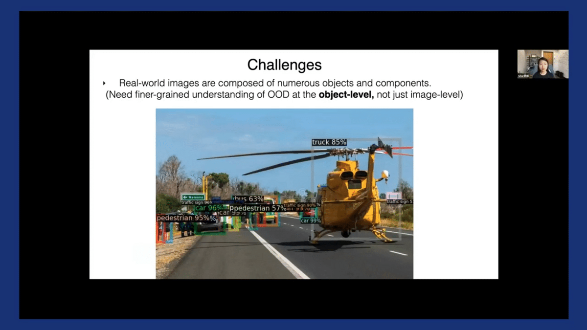
One last challenge is that real-world images are composed of multiple objects and components, and therefore we need a finer grain understanding of OOD at the object level—beyond the image level.
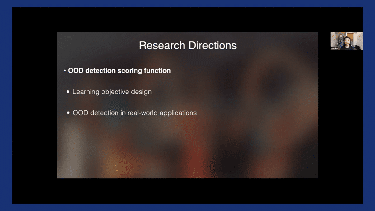
Here, I outline a few research directions that we have been pursuing, but there are also plenty of open problems out there. I roughly divide this into three parts—I’ll first talk about how to measure out-of-distribution uncertainty. Then, I’ll talk about learning objective design that can facilitate OOD detection. Lastly, I’ll talk about the connection to the real world.
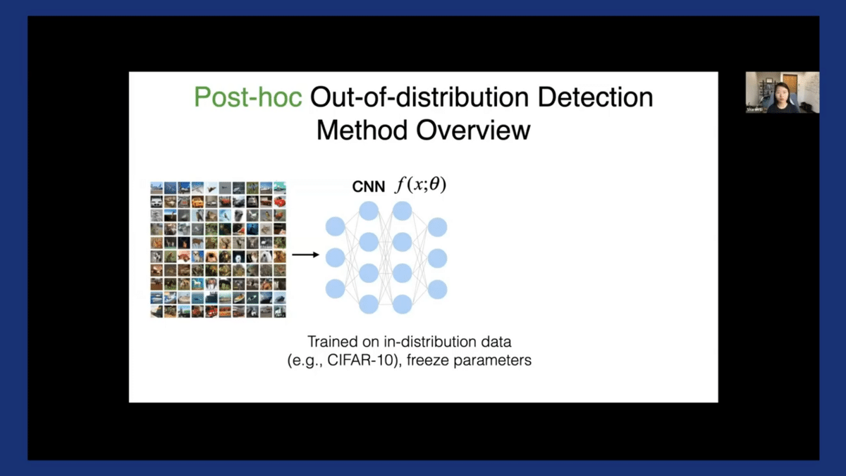
Let’s start with the scoring function. The earliest work adopted this post hoc approach for OOD detection. Here a model is typically trained on the in-distribution data, say CIFAR-10, using empirical risk minimization.
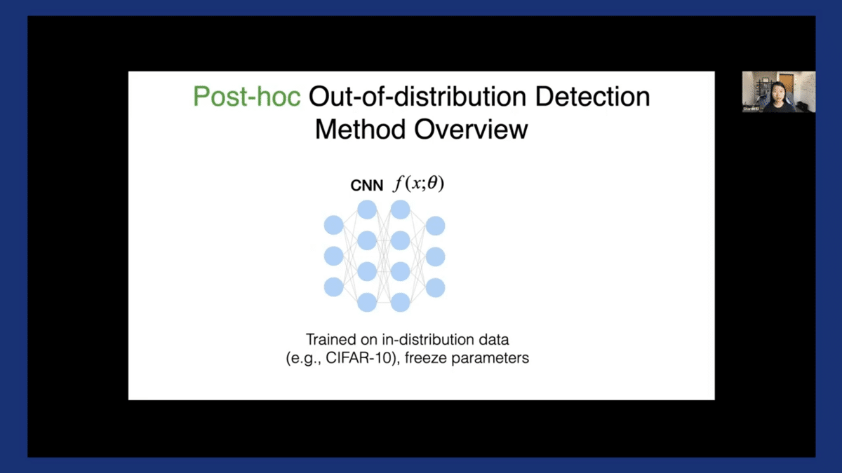
Once it’s trained, let’s take the network as it is, without modifying its parameters. During inference time for any given input, we are going to devise a scoring function. Let’s call this S for detection. Essentially we’re performing a level set estimation. If the score is below a certain threshold, we are going to reject this input. Otherwise, we’ll produce the class prediction as usual.
The advantage of post hoc OOD detection is that it doesn’t interfere with our original task. Therefore, the model can guarantee to have the same performance in classification while having this additional safety layer almost for free. I also want to note that the problem is different from the anomaly detection problem, which is also a classic machine-learning problem that treats all the data as one class without necessarily differentiating the class labels.
OOD detection often cares about achieving two goals simultaneously. We want to be able to classify or for multi-class classification and, on top of that, distinguish ID versus OOD.
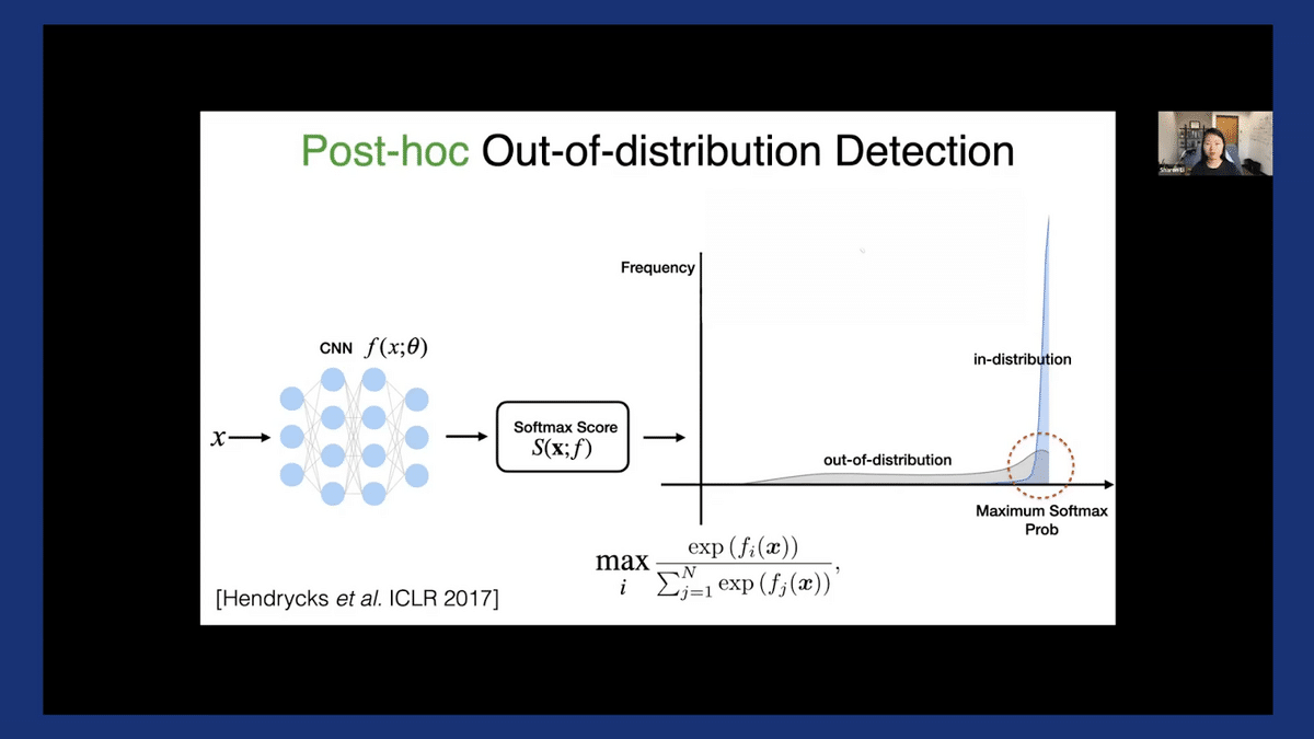
A common baseline is to use the softmax confidence score, which is also the largest posterior probability from the model. However, it doesn’t really work well because your networks tend to produce these overconfident predictions as we saw earlier. As is highlighted in the red circle, for both ID and OOD there is a non-trivial fraction of data that can produce this maximum Softmax probability, close to 1. You can’t reliably draw a threshold somewhere and separate these two types of data.
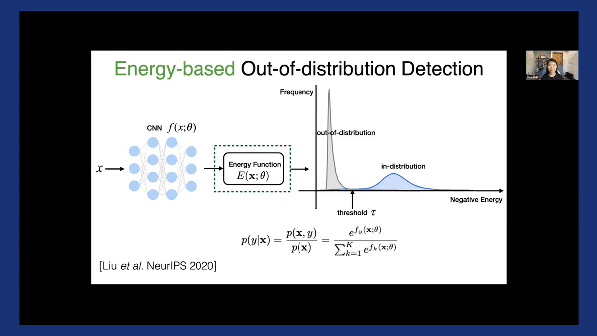
In our NeurlPS 2020 paper, we put forward an energy-based OOD detection framework, which has the core idea that influenced many of our recent works and other researchers as well. I see this as an important milestone because it really brings a new perspective to the community. Compared to the confidence score, we show that an energy-based score can better perform OOD detection, both in theory and empirically as well.
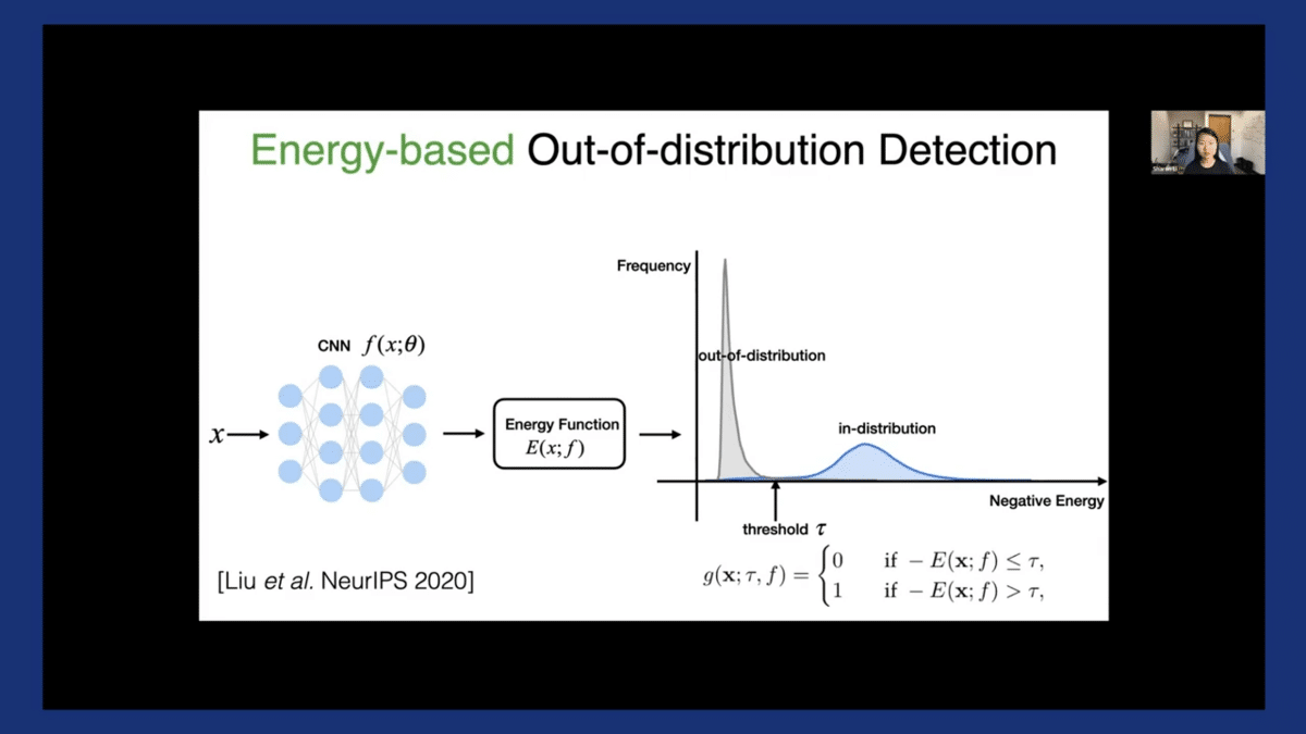
Here is the high-level view. Let’s say we have our input which goes through the network parameterized by theta. Then, we calculate this energy score, which I’ll talk about the definition in the next slide coming up. Once we have the energy score, we perform this threshold in comparison. If it’s smaller than this threshold Tao, we’re gonna reject this input.
Here, we flip the sign. This x-axis is based on negative energy, just to align with the convention that a larger score indicates in-distribution and vice versa.
So, how do we calculate the energy score?
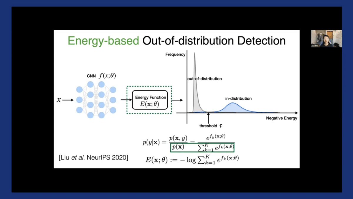
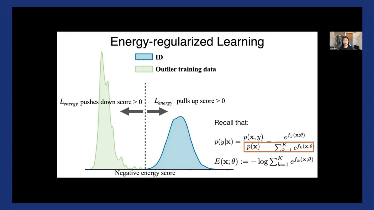
I would like to first remind you, this is the standard definition of the softmax function where the probability for an input to be associated with label Y—p(y|x)—is given in this form. The middle part of the equation is to rewrite this in terms of the joint probability divided by the likelihood of p(x). Now, we can connect the definition to this equation here. Energy score is the negative of the log of the denominator in the Softmax function.
As you can see here, energy has this inherent connection to this log-likelihood. We’ll come back to this connection, but I just wanted to signpost this here.
With energy score, the distributions become much more separable. As you can see here, the purple indicating in-distribution and the gray indicating OOD, we can draw this threshold and separate them much more reliably.
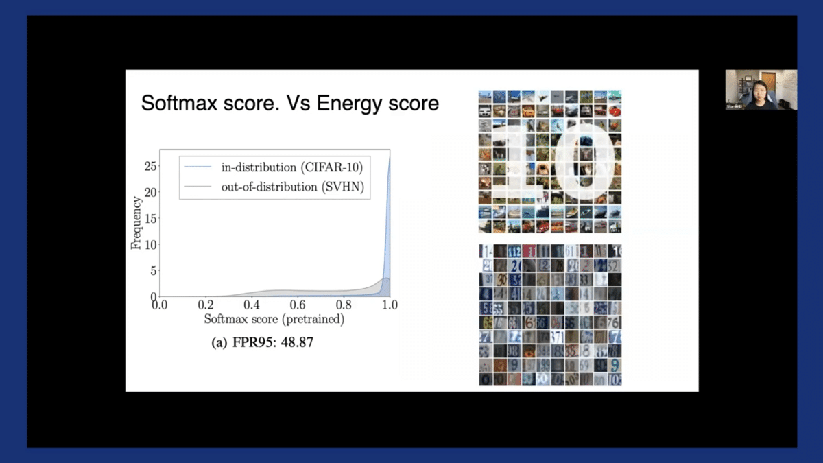
To evaluate and compare this approach with the softmax score, here we train a model on CIFAR10 as in-distribution and evaluate on SVHN as OOD.
The plot on the left-hand side shows the performance in terms of FPR (false positive rate) using softmax score. We measure the performance in terms of the fraction of OOD that is misclassified as in-distribution when we set the threshold so that 95% of in-distribution is above the threshold.
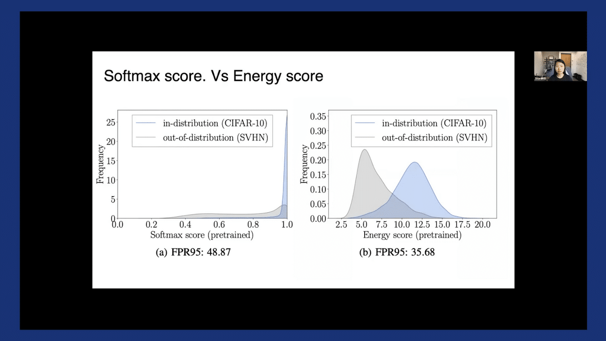
Lower is better. Here we see the FPR is around 48.87%. In contrast, using energy score can substantially reduce the FPR to about 35%.
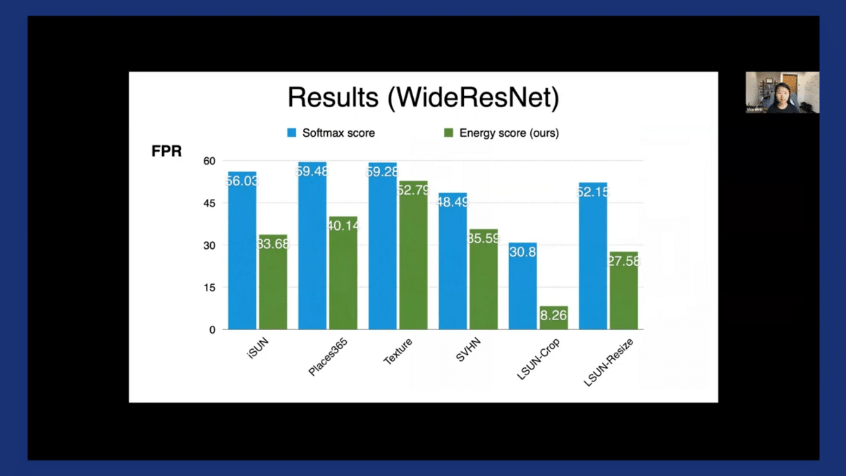
We tested fully on more OOD data sets and consistently observe a significant improvement. This is a model trained on CIFAR-10, and the X-axis highlights different OOD data sets. The blue is when we use softmax score, and the green is when we use energy score.
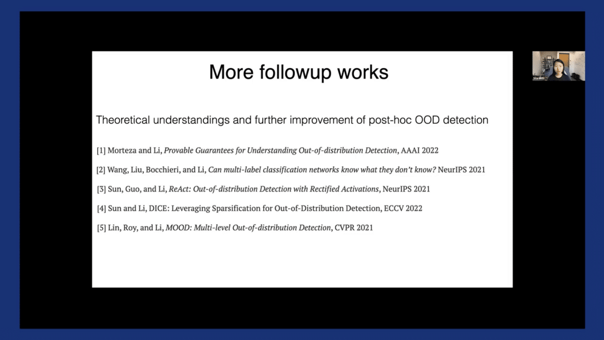
This paper has led to a series of follow-up papers as well. I wanted to show some of the high-level connections and summaries. For example, we provided provable guarantees of energy score in the first paper listed here, by Peyman Mortez and Yixuan Li. We also showed that energy can be extended to other learning tasks beyond multi-class classification, such as multi-label classification when each image can have multiple ground truth labels.
There are other follow-up works that showed, for example, using rectified activation and sparsification can further improve the performance of energy score. If you’re interested, feel free to check the works out.
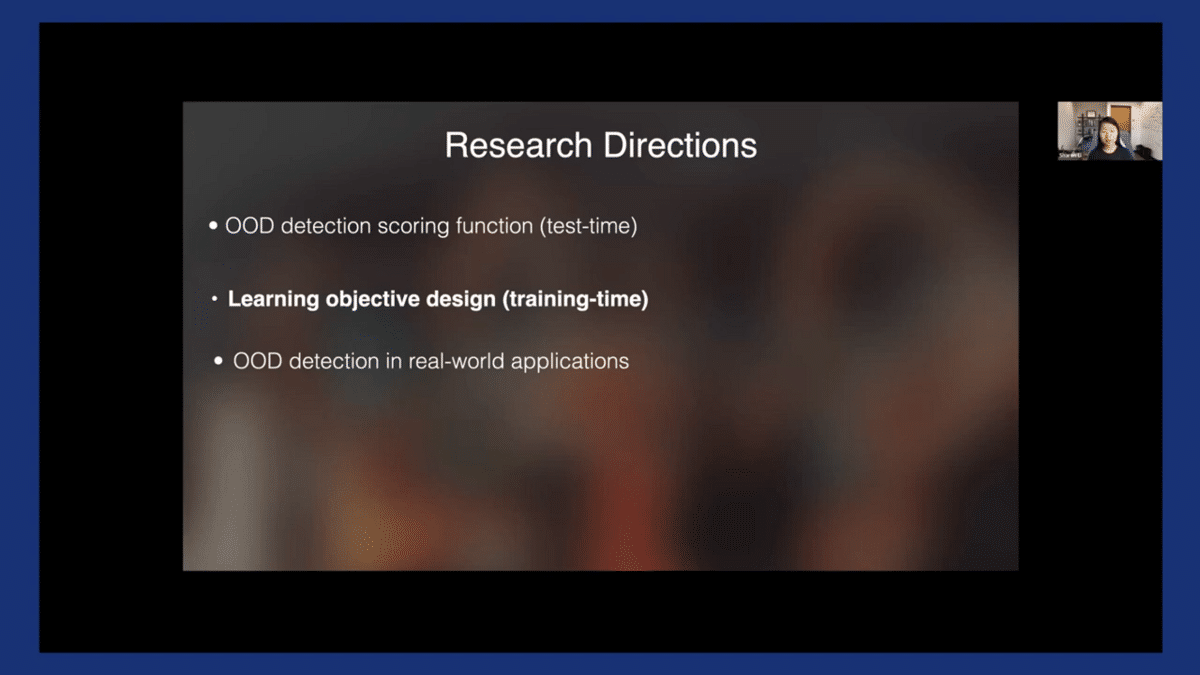
Going beyond the test-time OOD scoring function, I also want to briefly talk about the learning objective design from a training-time perspective. In my view, I don’t think we can fundamentally address this problem without rethinking how machine learning models are trained.
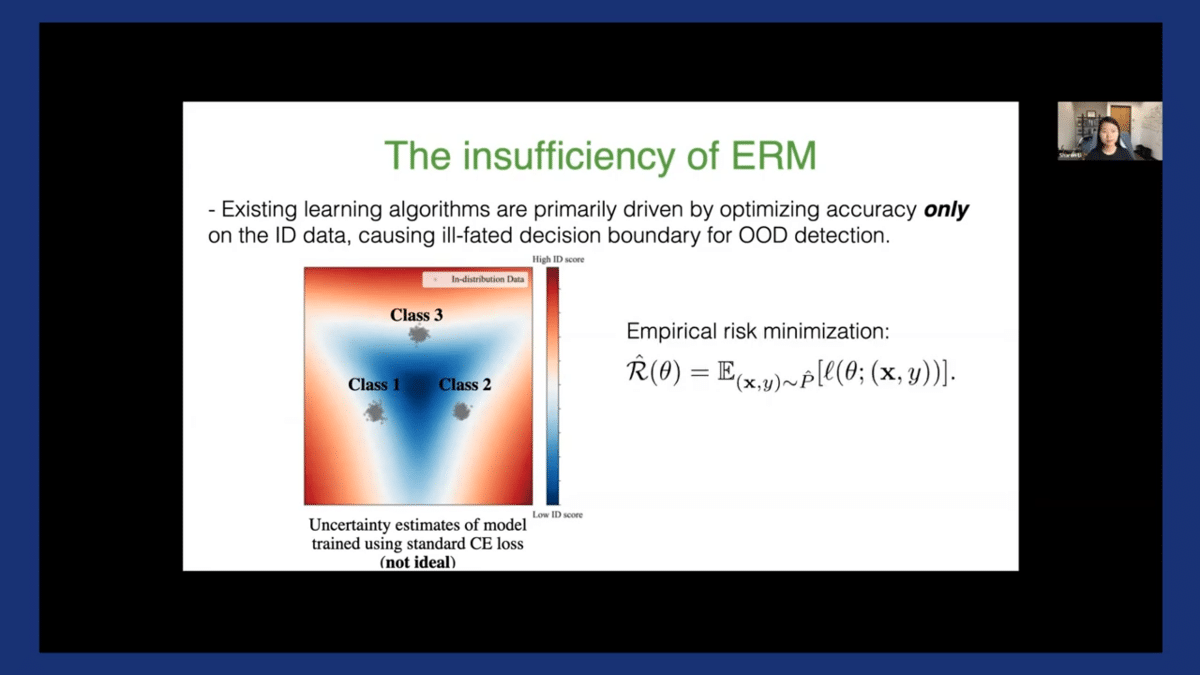
To explain what I mean, let’s revisit this example. This is a model trained using ERM on the in-distribution data only. The decision boundary, as we saw earlier, is good for classification but insufficient for OOD detection purposes.
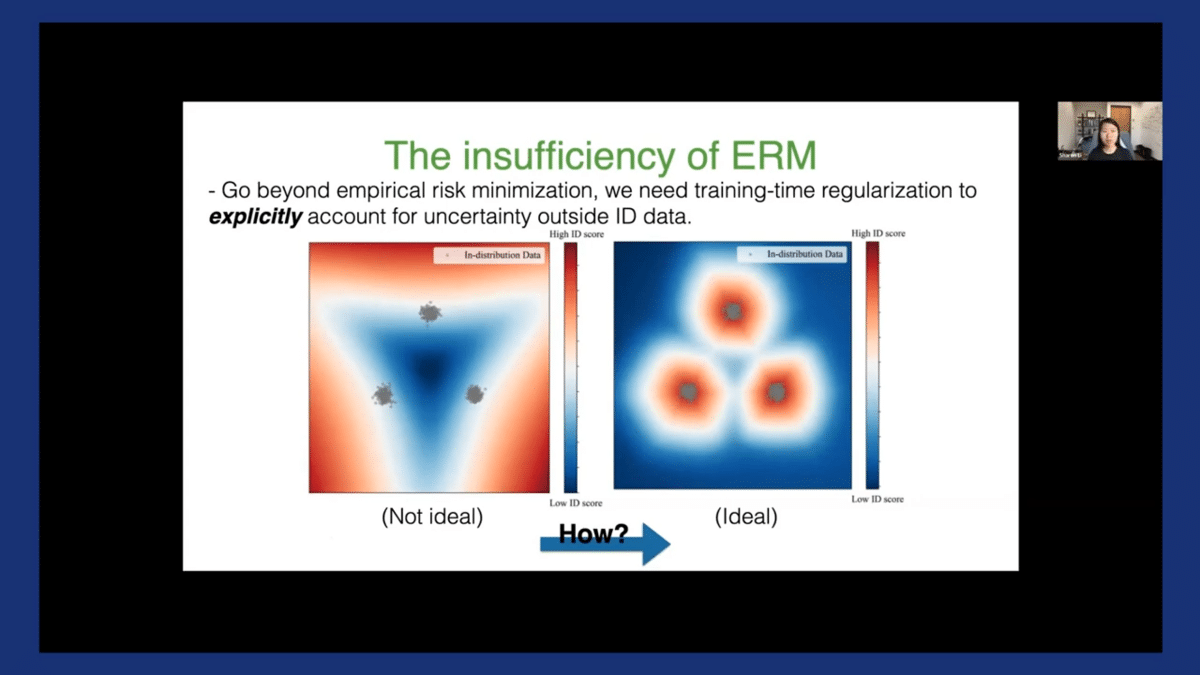
We need some training time regularization to explicitly account for the uncertainty outside the in-distribution data. The ideal decision boundary should be something more like the right-hand side—that’s much more conservative surrounding our in-distribution data. The question really is, how do we go from the left to the right side?
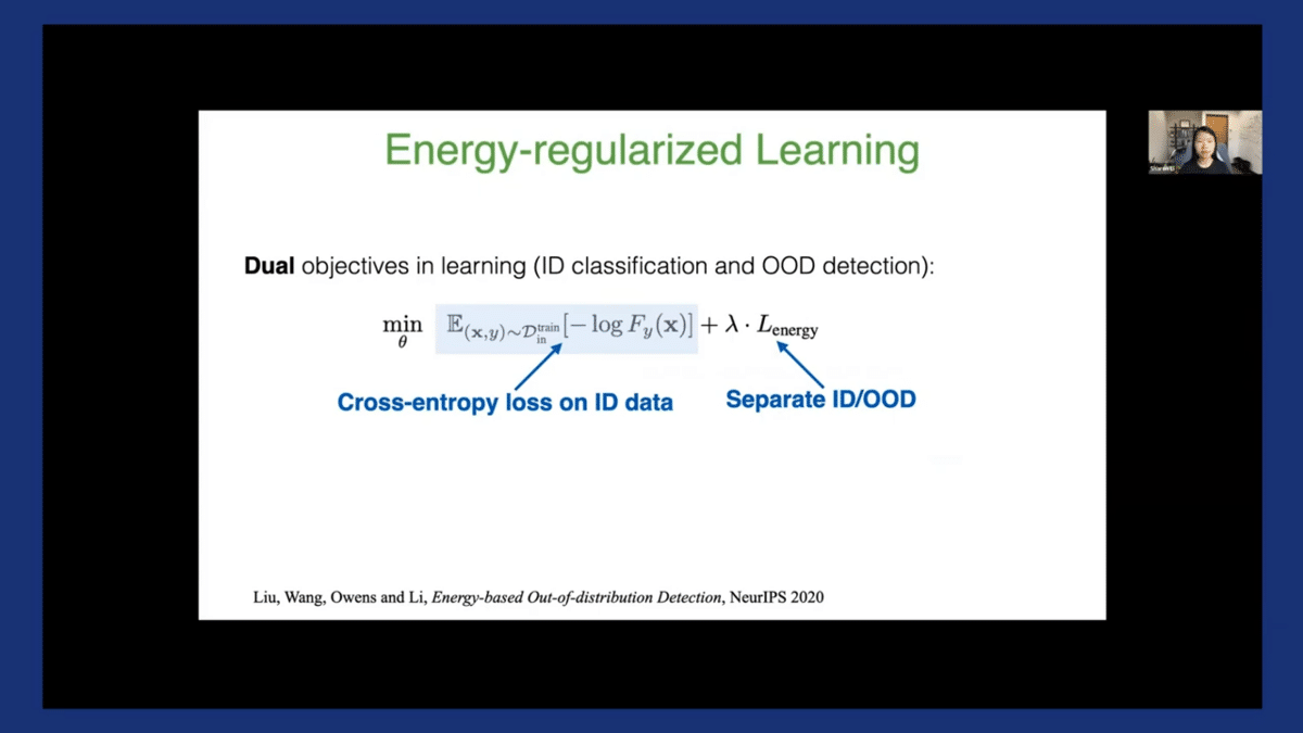
To do so, we advocate for dual objectives in learning. It’s a combination of the standard cross-entropy loss which tries to classify the ID data. Additionally, we have this uncertainty regularization term, Lenergy, that tries to separate ID versus OOD data. The right-hand side, the second term is the new thing here.
Now, let’s zoom into this regularization term, Lenergy.
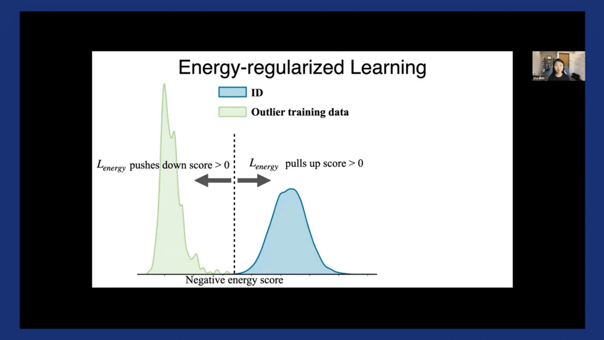
Here’s how it works. For now, let’s assume we have access to some auxiliary outlier training data (I’ll talk about how we relax this assumption in a second). Once we have that, our key idea is to explicitly push the energy score to be on two sides—basically, threshold it at zero. This middle dash line is when the energy is zero, and we try to push the energy scores to be on the two sides of it for ID versus OOD.
This objective has some nice mathematical interpretations too. Essentially, we’re performing a level-set estimation based on this measurement of energy score, which is related to the log-likelihood. This optimization is also much simpler and easier to optimize than directly estimating the log-likelihood, which can often be intractable.
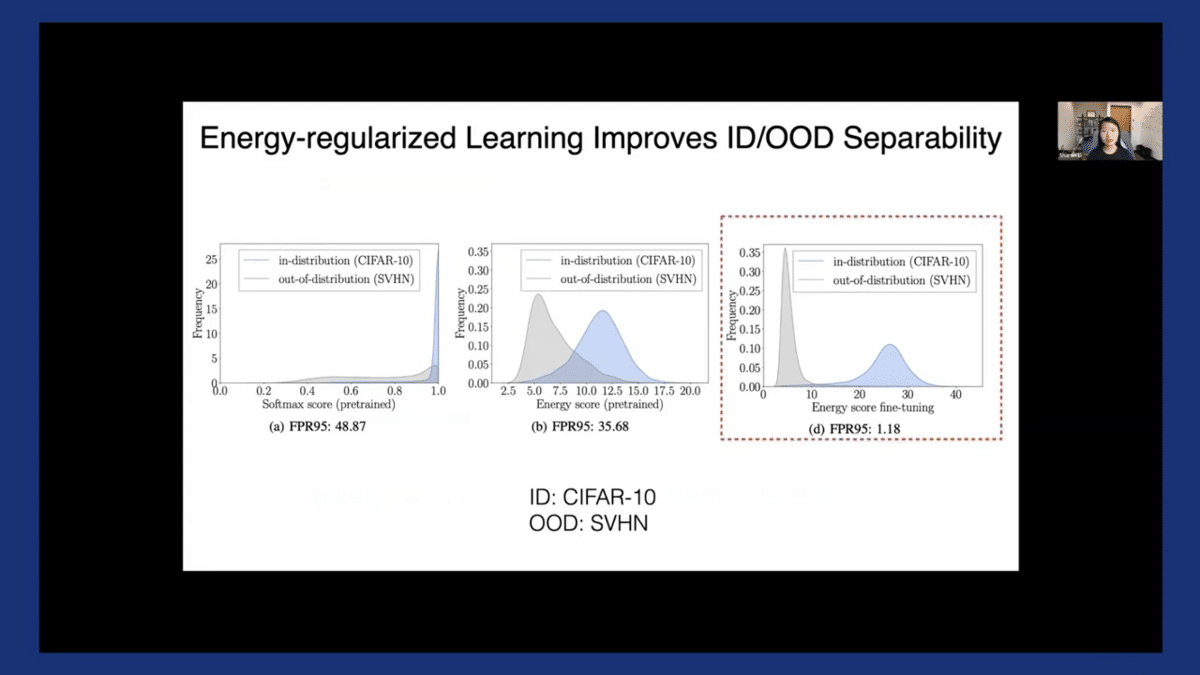
The result of the training is more separable distributions measured by energy score, as you see on the right-hand side where the FPR can be further reduced significantly.
This framework also opens up some interesting research opportunities and open questions. For example, I have previously mentioned that the framework may assume that we have access to some auxiliary outlier data, but where do we even get the data from?
One idea to think about is: can we leverage this wild data that we can naturally collect upon deploying a machine learning classifier in the wild? At a high level, this wild data can offer several advantages. For example, it better matches this true test-time distribution than using data collected offline, such as web crowd images. Secondly, this approach doesn’t require manual data collection. You can get a lot of data in abundance.
However, the challenge here is that the wild data is not pure. It’s a mixture of in-distribution and OOD. The interesting research question here is, how do we get around this issue? If you’re interested in these questions, please check out our ICML papers that are coming out this year for methodologies for working around this and some theoretical guarantees.
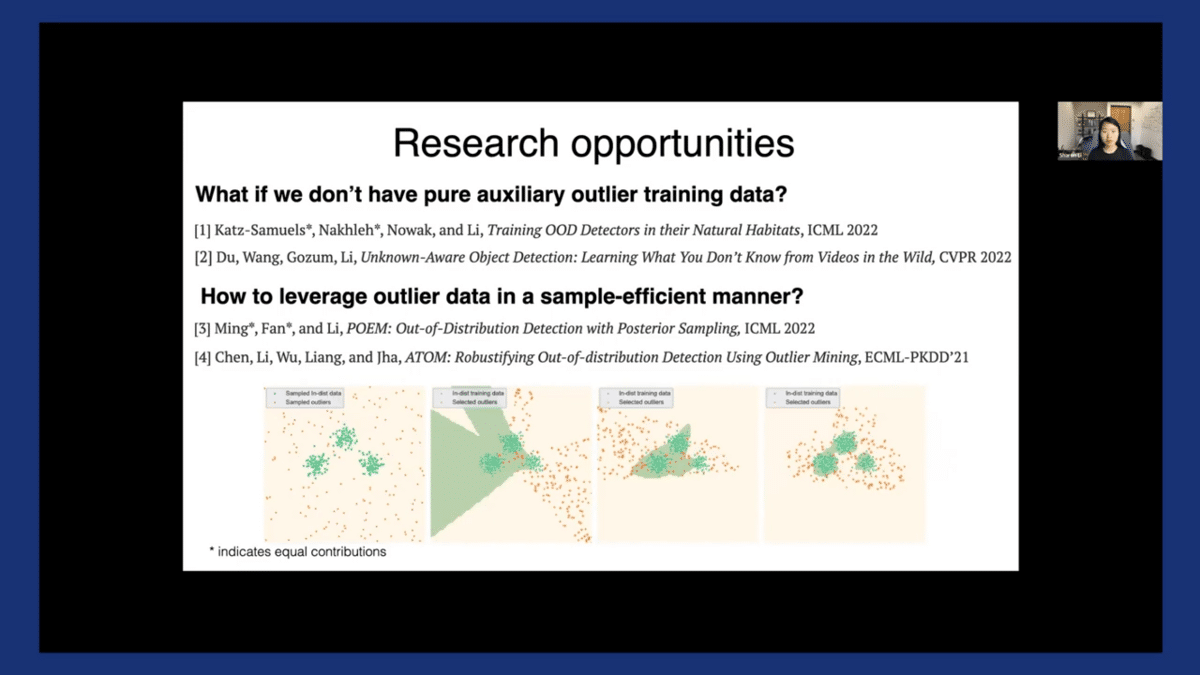
Another related research question is, how do we leverage this outlier data in some sample-efficient manner? This is particularly useful when we are dealing with a very large sample space of outlier data. We put forward this notion of outlier mining which aims to identify those most informative outlier training data points that are sufficiently close to the decision boundary between ID versus OOD, as you see in this figure.
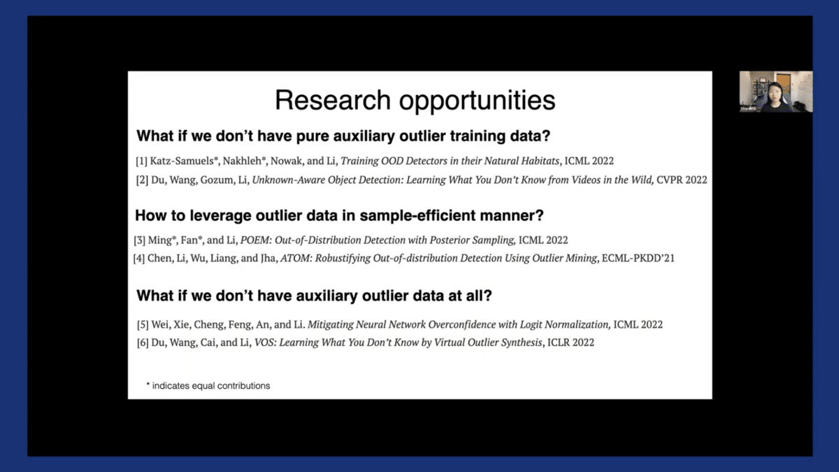
Lastly, what if we don’t have any auxiliary outlier data at all? When it’s not feasible or possible to collect any, what can we do? Is there something smart we can achieve just by working within in-distribution data itself?
I just wanted to briefly touch on this connection to the real world. When we’re deploying these out-of-distribution detection methods for the real world, there are a couple of important considerations.
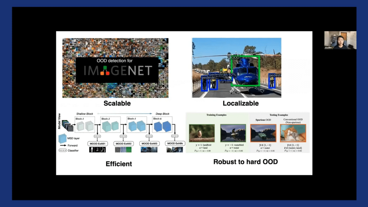
The first is scalability. For example, a lot of these approaches have been commonly benchmarked on simple data sets, such as CIFAR, which have relatively lower resolution and fewer classes. In the real world, we’re going to be dealing with much higher-resolution images with a lot more classes. How do we scale up OOD detection methods to this large-scale setting? It’s a very important problem to work on.
The second is this localization ability which, as I mentioned earlier on in this talk, we need a finer-grained notion of OOD at this object level, beyond the image level. For example, in the above image, all we wanted to highlight is this helicopter as “unknown”, whereas the pedestrian cars and all the other objects are still normal in-distribution objects.
Efficiency is another important consideration, which could matter in safety-critical scenarios where latency matters. For example, in the case of a self-driving car being able to detect OOD in a computationally efficient manner can potentially caution the driver far in advance. We need some efficient methods for detecting OOD with high accuracy as well.
Catch the sessions you missed!
The Future of Data-Centric AI 2023, our two-day free virtual conference, brought together thousands of data scientists, AI/ML practitioners, researchers, and the AI community at large to hear about and discuss the latest trends and research in data-centric AI. If you registered for the event but didn't see all the sessions you wanted, you can now catch up. The recorded sessions are available for registrants at the same Zoom portal as the live sessions.

Team Snorkel