
Understanding the label model. Machine learning whiteboard (MLW) open-source series
Background
Frederic Sala, is an assistant professor at the University of Wisconsin-Madison, and a research scientist at Snorkel AI. Previously, he was a postdoc in Chris Re’s lab at Stanford. His research focuses on data-driven systems and weak supervision.
In this talk, Fred focuses on weak supervision modeling. This machine learning whiteboard episode is part of the #ML whiteboard video series hosted by Snorkel AI. Check out the episode here or on Youtube.
Additionally, a lightly edited transcript of the presentation is below.
Weak supervision modeling pipeline
I figured we’d do a quick presentation on trying to understand the label model and what it’s really trying to do, so that when you check out the code, you can make sense of what’s actually happening there. I’ll try to make this as intuitive as possible. There’s some math, but hopefully, it’s not “really bad math.” If I’m going too low-level let me know and we’ll explain things. If I’m going too high-level, also let me know and we’ll talk more technically about stuff.
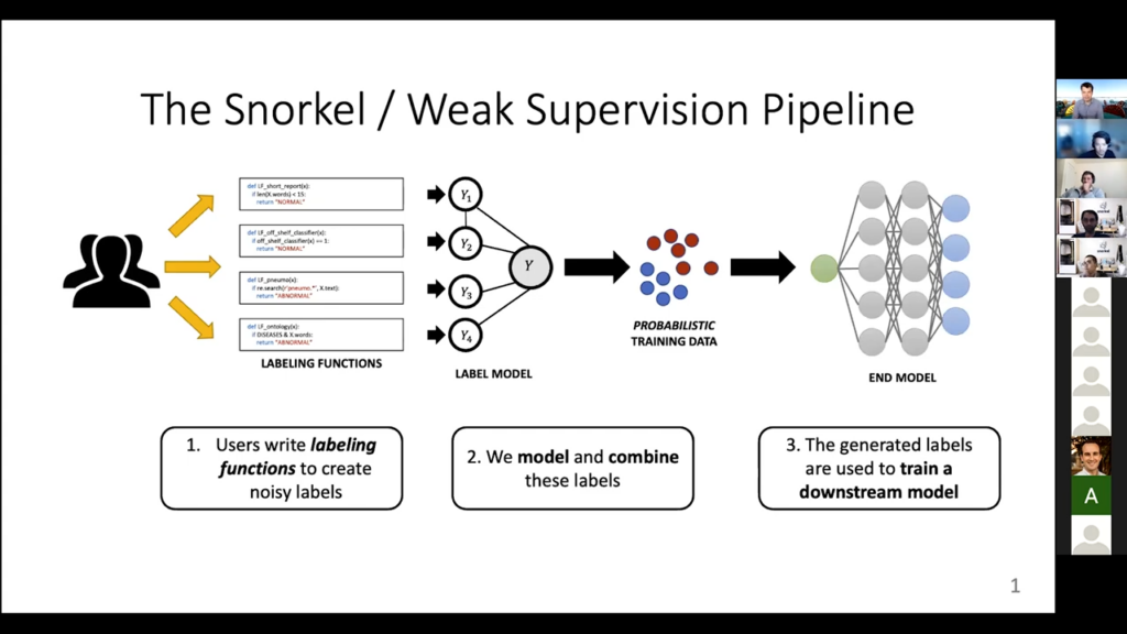
So this thing, which you’ve probably seen before, is our traditional Snorkel weak supervision pipeline. Currently, Snorkel actually does a lot more than this, but this was sort of the original vision. You have the users who write the labeling functions, which can be roughly anything. Then these labeling functions get applied to some unlabeled data points and they all provide some conflicting and probably noisy guesses of what an unlabeled data point should be. Then we try to figure out how to model the labeling functions. So: how to know which ones are reliable, which ones are not reliable, which ones I should sort of throw out or not, and what do we do with them. By doing that we can figure out the best guess of what the actual label should be, and that provides us with this automatically constructed data set. We then train some and model on that. So that is the standard picture. We’re going to talk [today] pretty much entirely about this second phase, the label model itself.
Understanding the label model
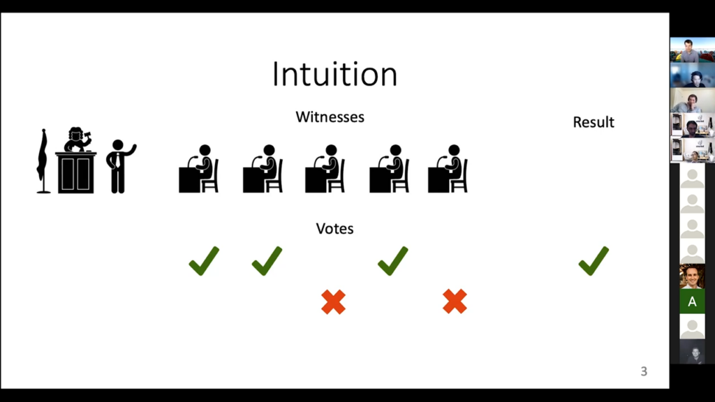
What’s the intuition behind what we’re doing for the label model? The picture I always come up with is that: you’re in a courtroom. We always talk about the “true” label for a data point as being this latent, unobserved variable, and that’s exactly what happens in court. You don’t know whether the person who’s accused of a crime actually committed the crime or not. If you were confident—if you already knew—you wouldn’t really need a court procedure. But you don’t really know so you have to use some alternative forms of information to try to guess what the case is.
So this is the courtroom and the thing that we get information from are these witnesses. Each witness will say, “I think the person who’s accused committed the crime” or not. In practice, it’s a bit more complicated than that, but let’s go [with] this really simplified analogy. These witnesses are kind of like our labeling functions. This variable of whether it was a crime or not is kind of like a plus-one-minus-one label for our case. One witness is plus one, one witness is plus one, one witness is minus one, or whatever. The easiest thing to do is to then say, “okay well let’s look at what the majority of the witnesses say.” If they say that there was a crime let’s go with that. If they say there was no crime, then let’s just also go with that. That’s the standard thing to do, and this is exactly what the majority-vote aspect of the label model is also doing. It literally says, “okay the majority of the labeling function said plus one, let me say this data point is a plus one.” If the majority said minus one, then it is a minus one. This is a really simple case, [but it is] still really useful, actually. You can get a lot from doing this. But there are some downsides.
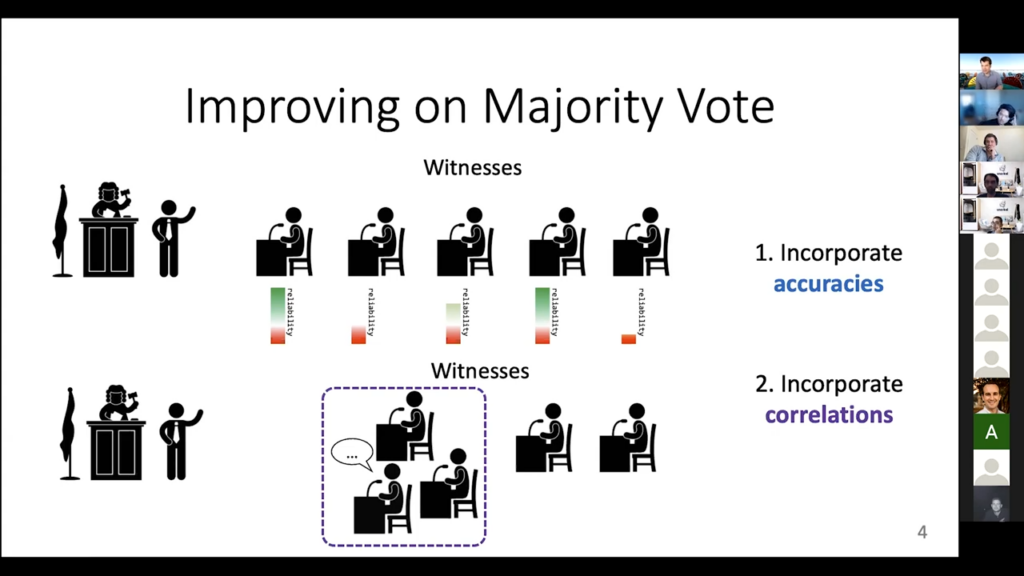
One downside is that all these [witnesses] are not equally reliable. Some are really reliable, [and] you can trust them. If they say there was a crime then there probably was one. Like this first one here. The other ones may not be as reliable. Maybe they don’t give you that much information. You don’t want to throw out the witnesses that are not as reliable, but you do want to find a way to weight them differently. You want to trust the reliable ones more than the unreliable ones, but the hard part is that you don’t know for sure who’s reliable and who’s unreliable. That information doesn’t come to us. We have to figure it out on our own. We call this “accuracies.” We want our label model to incorporate the accuracies of the labeling function.
The second [downside] is: imagine if three of the witnesses cooperated and talked together before we went to court. If they got their stories straight together, you wouldn’t really trust them as much as three separate independent people, because maybe they have different views but once they coordinated they’ve kind of come to agreement on one view. This is this problem of correlations or cliques. You’d like to be able to down-weight people who have gotten their story straight beforehand.
These are the two things that we really want our label model to include over majority vote. The majority vote doesn’t know how to deal with any of these problems. It gives equal weight to everybody, reliable or unreliable, and it gives equal weight to everybody even if they form the clique and discuss in advance, or whatever the analogy is here. So, we want to include these two things in our label model, which means we will have to learn about these accuracies and these correlations.
I promise I won’t have any more silly analogies or images from this point on. Let’s get into the kind of actual modeling for these things. The math for it is this notation, “lambda 1,” “lambda 2,” through “lambda n.” These are the labeling functions. They’re random variables, they take on values like “minus one” or “plus one.” Then, of course, there is this true but unobserved label “Y.” We don’t get to see it, but it’s there.
How do we model the setup?
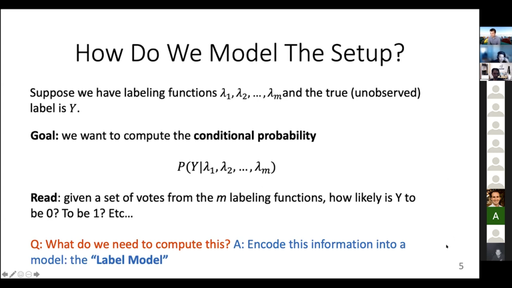
What’s our actual goal in this case? Very concretely, we want to compute this probability P(Y) given lambda 1 lambda 2 through lambda n, so this is a conditional probability. It is the probability of the label having known that we have this information from the labeling functions. You can read it as saying: what’s the probability, given all of the guesses that we’ve seen, that Y has value 0 or 1 or 2 or whatever. This is already much nicer than, say, the majority vote, because we don’t have to just say, “oh yeah, I think it’s plus one.” I can say, “yeah, I think it’s a probability of 0.6 of being plus one and 0.3 of being minus one,” and so on. That’s a lot more useful information that you can give to your model when you’re training instead of just saying, “has to be a plus one because the majority of the people said this.”
So, we want to compute this conditional probability. The hard part is we have to know enough information to actually compute it, and the way we’re going to do that is by encoding all of that information into this model that we call the label model. That’s all the labeled model really is: all of the information that we need to compute these conditional probabilities that tell us, given what the labeling functions output [is], what do we think is the probability of every possible value of the true label? Does this make sense—is everyone sort of happy with this formulation? And, we haven’t really done anything yet here, we’re just defining what the problem is and where we’re trying to go.
What’s a machine learning model?
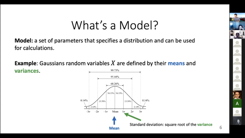
A machine learning model is a set of parameters that can fully specify some distribution, that you can then use for calculations. I want to be able to compute this conditional probability, so I need a model that gives me enough information to compute that. And that’s it.
There are a lot of different usages of models in Snorkel, so we have to distinguish between the different ones here. A really simple example of a Gaussian random variable, you can think of it as a model just by itself if [you know the mean and if you know] the variance, that is all you need to know about it. It completely specifies the entire distribution for a Gaussian. So, if I tell you the mean and the variance, you can say, “oh yeah, the probability that X equals 3.7 is this much; the probability that X is between -2 and 16 is this much,” and so on. You know all the information to compute stuff like that.
For our label model, we want to define similar things. We want to find: what are the parameters that are going to be enough for us to compute these conditional probabilities for the true label. Here’s the classic image of the bell curve. The mean is the thing in the middle. The standard deviation is the square root of the variance. It’s like sixty-whatever-eight percent off or whatever it is for this kind of thing. So that’s the model idea.
Random Variables
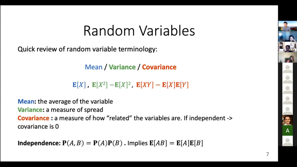
I’m already talking about random variables, so let me briefly remind you of some of the notation—I’m trying to stay away from any really deep math but we’ll need this part, unfortunately. The mean is just the average. That’s this expectation of X. The variance is this measure of the spread—how far away you are from the mean, on average. The really interesting one that we’ll use a lot is this covariance between two variables. It is kind of a measure of how related two variables are. [When] variables are independent, which means they have no information about each other, their covariance is zero. We’ll use this quite a bit. You can already kind of think of this as defining an accuracy. Like, we want to know the covariance between one labeling function and [the] true label. If a labeling function is really bad at guessing the true label, the covariance between these two things will be zero. And then finally, there’s this independence property, which is the classic one that we always talk about. A and B are independent if, and only if, P(AB) is P(A) times P(B). And this implies that the expectations for these two things you can write the product as the product of the expectations. Nothing crazy going on, just basic probability stuff from back in any of these classes.
Setting up the model
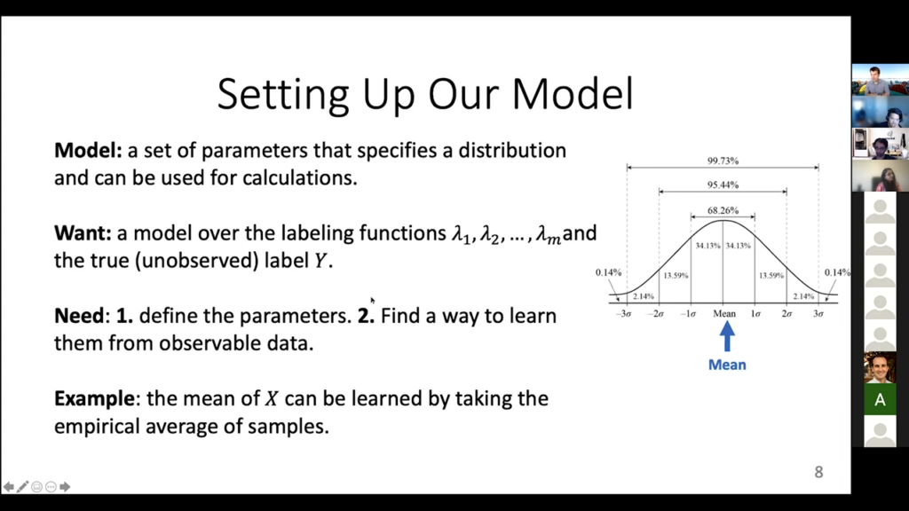
Now we’re going to set up the model that actually is the label model itself. Again, these are just some parameters that specify the distribution that we’re going to use to compute this conditional probability. It’s going to have to involve all of these variables, the labeling functions in the true unobserved label, and then of course we’re going to have to learn these parameters from data, because we don’t know them a priori. In this Gaussian case, for example, you could compute the mean by just taking a bunch of samples, adding them up, and normalizing, dividing by how many things you saw. We are going to have to find a similar way to do stuff here, as well. You can think of a coin flip in the same way. If the probability of heads is P, you could estimate P by flipping a coin 10,000 times, seeing how many heads there were, and dividing by 10,000. That’s an empirical estimate of P. We have to do a very similar thing for us too, okay?
So, just recapping, so far we want to go beyond the majority vote by integrating these kinds of accuracies of the labeling functions and possibly how correlated they are. To do this, we have to introduce some statistical model over the labeling functions in the true label. We have to figure out: what are the appropriate parameters that encode all this information? We have to figure out a way to learn these parameters. And then we have to find what calculation is going to give us that conditional probability. What is the probability of the true label, given what we saw from the wavelength functions? That’s the current game plan.
So with this, we can write down the label model for each of the witnesses, or whatever. We just have one of these nodes. Everything is written in this format of a graphical model. It’s not super important yet, but it’s a very convenient way for us to specify what these things look like. There is one node for each labeling function. There is a node for the true label, Y. We won’t ever get to see Y. That’s the whole idea behind weak supervision. We will see samples from the labeling functions, that’s the information we get to use.
Specifying the label model parameters
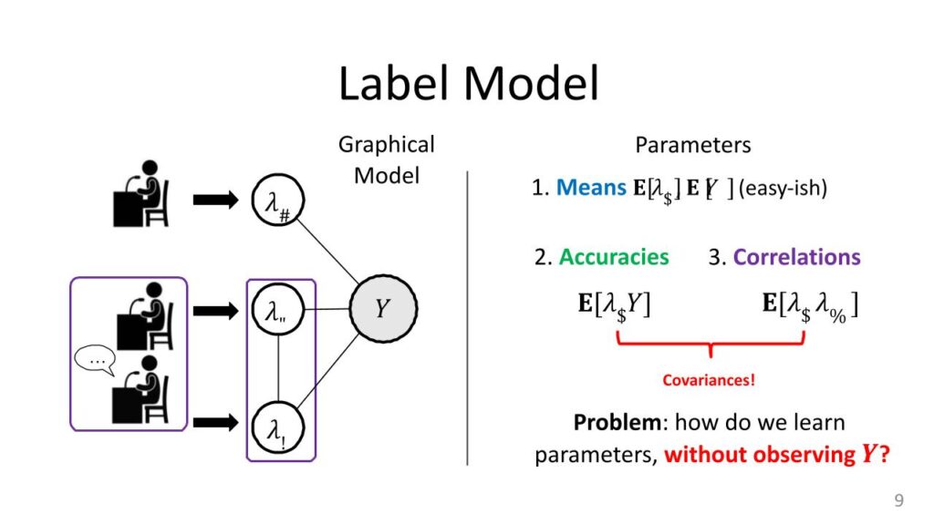
Now, let’s specify what these parameters are actually going to be. Obviously, we want things like the means, so the expectations of each of these labeling functions, lambda I, also the expectation of Y. These things are easy-ish to estimate. The expectation of lambda I is just: look at all of the labeling function outputs for the If labeling function, and then see how often it votes one, how often it votes minus-one, divided by the total, [and] that gives you the mean. The expectation of Y is harder because you don’t get to see the true labels, but you can get this too if you have, say, a dev set. You just get an estimate of the class balance from a dev set and there are other ways to do this as well. These are the means, and if you remember that Gaussian case, the means and the variances give you everything. It’s going to be the same thing here as well. The variances or covariances are going to be these accuracies and these correlations. The expectation of lambda I times Y, and then the expectations of this product lambda I comes lambda J.
Assume we’re talking about binary variables, here. So they are all either plus-one or minus-one. If your lambda I—your labeling function—is really accurate, then it’s going to always agree with Y. So when Y is one, it’s going to be one. When Y is minus-one, it’s going to be minus-one. This product will always be one, because one times one is one and minus-one times minus-one is also one. This expectation is going to be close to one all the time. If they’re really inaccurate, you’re going to be close to zero all the time. This kind of parameter will tell us how accurate the actual labeling functions are, and that’s why we can justify this accuracy name. Correlations are the same things. How often do labeling functions agree with each other or how often do they disagree with each other? That’s actually all that’s going on here on the left, basically. Each of these edges between a random variable and Y is actually like one of these accuracy parameters. Then in the cases where there are these correlations—which was the whole labeling functions that are cooperating together—you’re going to get one correlation as well. This gives you all of the parameters of the model. Just like the Gaussians, you have these means, you have this covariance instead of variance, if you know these, actually you have enough information to compute those conditional probabilities from before. The goal for the label model is just to figure out these guys. If the label model can do that, then everything else kind of follows from here.
Now, the hard part, of course, it’s very difficult to do this compared to the coin flip example. This is a special case here the accuracies. Normally, if I was computing this mean, I would say, “let me get a bunch of samples and just kind of take their average.” But I don’t know what Y is here, so I can’t just take samples of lambda I times Y. That’s the hard part about weak supervision. You don’t know the true label, so you can’t easily compute these kinds of empirical expectations. That’s the only real trick that we’re going to have to use here for the label model. A way to get access to this information without actually knowing what Y is. That’s the whole setup label model is literally this system or distribution on the left, which has this kind of graphical representation. Nothing is happening here except having a bunch of parameters. We would like to learn these parameters. If we know them, we can get a really good estimate of what the true label should be from the labeling functions. If we don’t know these, we’re stuck with the majority vote, which may not be as precise as the label model’s full information.
Let’s get to the part where we actually get our accuracies, which is the biggest technical challenge here.
Graphical model review
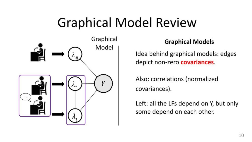
These graphical models that we were talking about, they’re not really critical for understanding what’s happening here. It’s just a convenient representation that tells you some information about these distributions by looking at this graph. In this graphical model, there’s a node for every random variable. The edges tell you something about correlations or covariances. There is a real technical explanation for what exactly they mean, but very roughly if there is an edge between things you can think of them as correlated. If there’s no edge between a pair of nodes, you can think of them as having some type of independence between them. Sometimes you have to do something to the variables to get out that independence, but that is the basic idea. In this setup, the labeling functions are always connected to the true label. If they were not, then there would be no relationship between the labeling function value and the label. You would have a “random guessing” labeling function, which would not be useful. We always have these edges between the actual value of the label and all the labeling functions.
Now, sometimes we have edges between pairs of labeling functions, and sometimes we don’t. When we have that pair, [it] is the case of correlations. That was in our whole jury setup when you have two of the witnesses talking to each other and coming up with the story. That’s something we also want to model because we do want to down-weight those values. And in fact implicitly when you compute this conditional “P(Y) given stuff” probability, you’re actually going to take that into account when you compute it.
Diving into the learning parameters
Exploiting independence
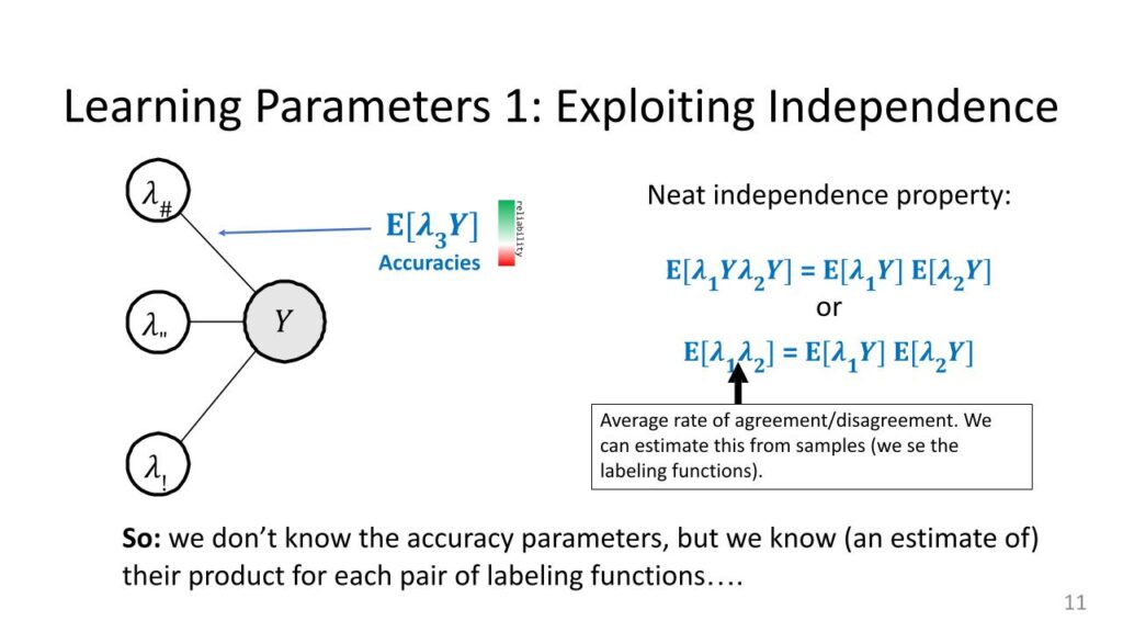
Here is the sort of first and maybe easiest method for learning the parameters. The only real parameter we care to know about is these accuracies. That is the one that’s hard. Everything else we can kind of do. So I’m going to exploit independence specifically, and that’s why [with] this graphical model on the left there are no edges between the labeling functions, only between lfs and the true label. Again, remember what these accuracy parameters are. There are these expectations of the product of a labeling function and why and sort of the bigger these are, the more reliable you can think of a labeling function. If they’re perfectly reliable I would just use that information for Y. If they’re super unreliable, we want to down-weight them.
Let’s look at this really neat property of independence. The labeling functions themselves are not independent of each other, which is good because they’re all trying to predict the same thing. If they were independent, they’d have to be terrible. But it turns out that the products of the labeling functions and Y, these things often are independent—essentially the accuracies are independent even though the variables themselves are not independent. So, what does that mean? If I write this product on the left, this lambda 1Y, lambda 2Y, I can factorize this product because of independence as the product of two expectations. It is: the expectation of the product is the product of the expectations. That’s one trick.
Triplets
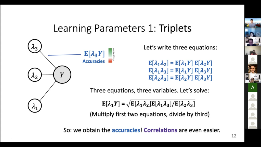
There’s a second trick. This Y was plus-one or minus-one. Those are the two possible values. When I multiply lambda 1Y lambda 2Y, I get lambda 1 lambda 2Y-squared. But Y-squared is one, regardless of whether Y is plus- or minus-one. This one just goes away. I end up just seeing lambda 1 lambda 2‘s expectation here. So, this is neat. We’re writing the expectation of lambda 1Y times lambda 2Y which are these two accuracy parameters. Their product is this correlation parameter that I can actually estimate. This thing is just the agreement or disagreement on average of a pair of labeling functions. If I look at all the things they’ve labeled, I can say: “oh yeah, they have the same label 75 percent of the time and they’re different 25 percent of the time and that tells me this expectation of lambda 1 lambda 2. In other words, this is observable. That is the key thing here. I don’t really know what the accuracy parameters are for these two labeling functions, but I do know that they multiply to be this kind of correlation parameter that I actually know. This is really nice. We don’t know the accuracy parameters but we know a function of the accuracy parameters, which is their product. This is actually the key thing that we have to have here. Once we have this, we can do a little system of equations. We can write down this exact thing for free labeling functions, just going two at a time. These three equations I just did this exact trick for lambda 1 lambda 2, and for lambda 1 lambda 3, then for lambda 2 lambda 3. Again, same idea. We have this independence property between each of these pairs. There are three different pairs and the cool thing now is basically that I have three equations and I have three variables. What are the three variables? They are just each of these accuracy parameters. I know the left-hand sides for all these cases, so you can think of this as A times B has some value, A times C has some value, B times C has some value. I know those three values and I need to compute A, B, and C from them. We can solve this. That’s [the] nice part.
How did I do this little solution? Take the first two equations and you multiply them. Both of them will have this expectation of lambda 1Y, so there’s a square there, and then I get times this guy, times that guy, then I divide by the third equation, which contains those two terms as well and they cancel out. So the only thing I will have left is this expectation squared. Then I take a square root. Okay, so a very “Algebra 2” level solution, here, but it’s really good. The accuracy parameter we were looking for, this one, is just equal to the square root of this expression, that involves three of the correlation parameters that we can actually get. So, even though we never got to see Y, and even though we can’t directly do a sample average to get this expectation, we have written it in terms that are observable. We can go [into] our label matrix and compute these three terms, solve this little equation here, and get our guess of this product. Then I can do this for every possible labeling function and I will get all of the accuracies. Correlation can estimate directly. I just do that sample average over all of them, just like the coin flips, so this slide kind of completes this process. Now we have access to all the accuracies and we are done.
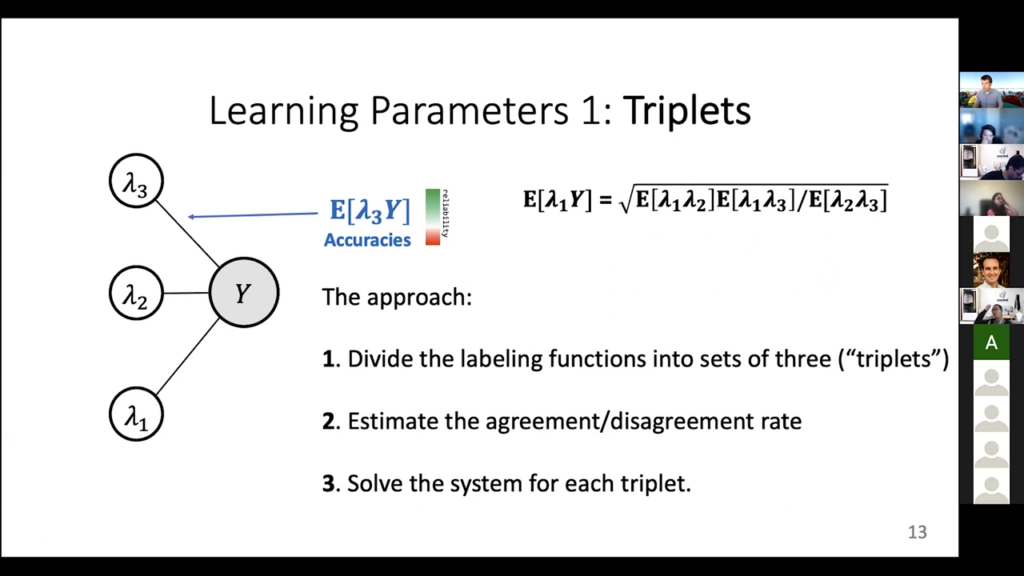
Let’s recap. The approach is [to] take all the labeling functions, split them up into sets of three, estimate these agreement/disagreement rates that you need, and then go ahead and solve the system for every single triplet. Once you do this, you have all the parameters, and this is actually what happens in one of the label model implementations. There is this fit method. It literally does this computation where it gets the accuracies and the correlations and once those are known there is a method that just does the inference step, which is this P(Y) given lambda 1 for lambda N: this actual probabilistic data thing that we want to get in the end. This is basically a full end-to-end, “how does the label model do what we need it to do,” kind of explanation. It’s not the default one, but it is one of the variants that we have implemented there and it’s really simple. I mean we didn’t really do anything here except compute one really simple formula to get all of the accuracy parameters, and then we’re done.
We are coming to it next. So just one second we’ll be there. Actually, I think it is the next slide. These are great questions.
Let’s also note the biggest downside of what we just did here, this little canceling trick of multiplying Y with itself, which is where we actually started. Here, we said that Y times Y is Y squared, which is always one. That is not true anymore if you have Y that could be more than plus- or minus-one. If it’s zero, one, two, three, four, then you don’t have this kind of equation any longer. So that is an annoying downside. This label model is very good for binary and not as good for higher cardinality cases.
Covariance matrix
Now we will talk about the most general version, which is this inverse covariance thing that we were referring to just now. This is the second kind of approach.
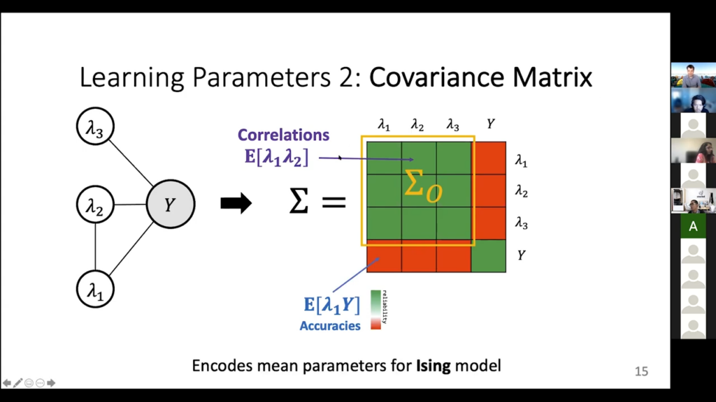
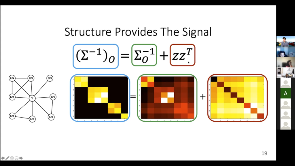
So, this is the second approach, which is a bit more general. It can handle a lot more stuff. It is also more computationally difficult. It is also the default thing that we actually do in the code currently. So far, we have talked about how all of these accuracy and correlation parameters are these covariances, and the nice thing is you can put all the covariances into a matrix because you’re computing the covariance of every node with every other node. And that is this overall matrix here. This green stuff is the correlations, which are the things of course I can directly estimate, and the stuff in red is, again, the accuracies that I cannot directly tell. So, nothing new here, just a new data structure for it, if you like.
Using graph-sparsity in inverse
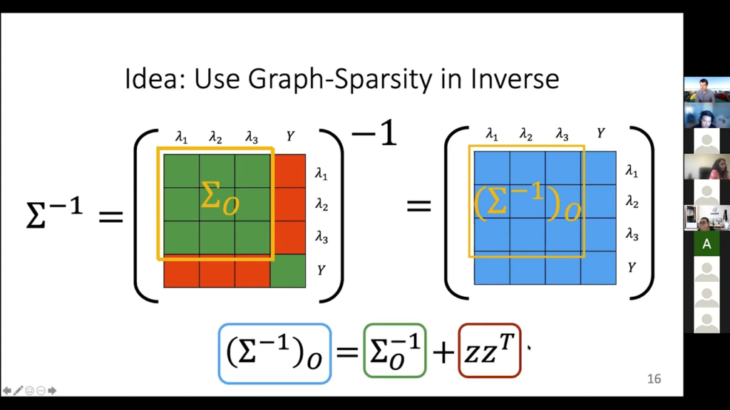
Now, there’s something magical that happens when you take the inverse of this covariance matrix. What is going on if we take the inverse? Basically, in the inverse it has something to do with the graph. Entries are zero if there is no edge in the graph that we have. Remember, not having edges in the graph was the sort of independence thing, and that turns out to reflect itself in the inverse covariance matrix. It is a very deep “stats” property. Of course, I can’t compute the full inverse directly, because I don’t know the red stuff, so I can’t just form a big matrix and then run NumPy inverse on it, at least not yet. I do know the full green part, though, and I can invert that. But inverting the green part by itself does not give me this yellow part of the inverse, like if you take a sub matrix and invert it, it’s not the same thing as that part of the full inverse matrix. But it’s close to it. It satisfies this matrix equation.
This looks confusing, but it’s not anything super crazy. All we are saying here is that if I take this yellow square of the inverse matrix—that is the left-hand side here—it is the same thing as inverting this green, known part of the forward matrix, inverting it by itself, plus one term that has to do with this red stuff, here. One more time: I care about this covariance matrix inverse because it has some special structure information. There are entries that are zero if we have this no edge between them in the graph, and I can also write down what this particular yellow component of the inverse matrix looks like. It is this left-hand term. I can express it as something that I know how to compute, plus some stuff that contains the parameters we care about. Now I’ve encoded all the information I care to solve into this matrix equation sigma inverse O, which is the observed part and is equal to sigma O inverse plus some stuff that involves the actual accuracy parameters.
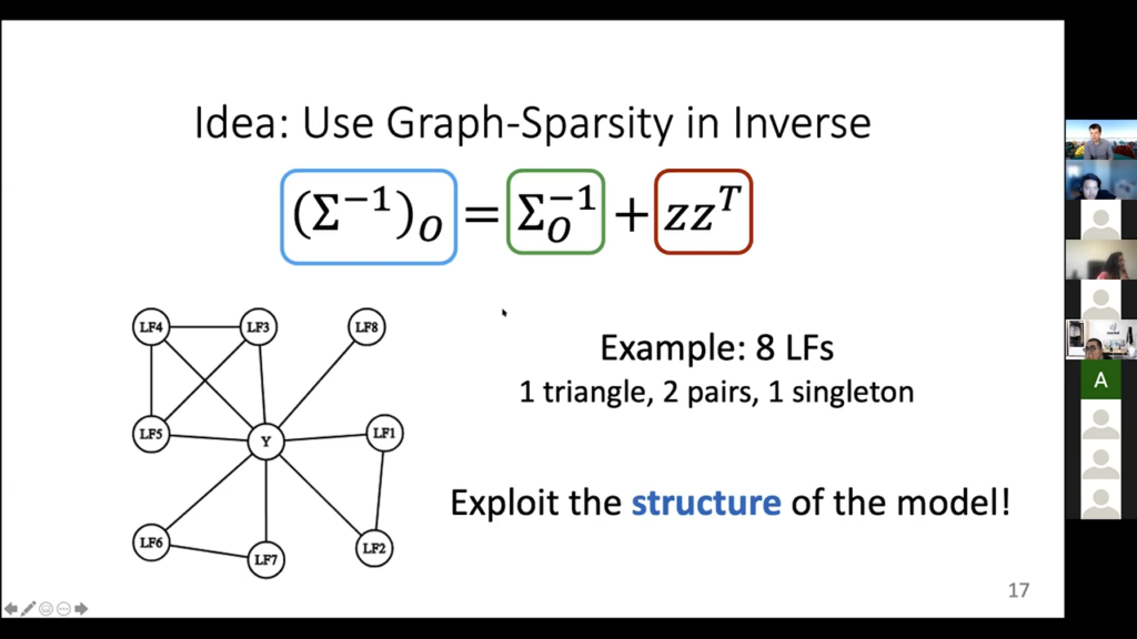
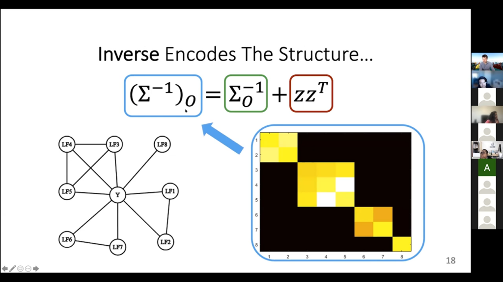
So that [is] high level, but we can show the actual details there. Let’s say this is the graph. We have labeling functions that are sometimes independent, sometimes not. There are some triangles here. There are some pairs. There is a singleton, which is this LF-eight here. We are going to use this information because of this whole “zeros in the inverse” covariance matrix. So let’s draw it out. Here is the inverse covariance matrix, this left hand side thing. Here’s what it actually looks like. These colors are the intensities of the values. Black means zero, so why are there these black parts off the diagonal? Well it is precisely because there are no edges between labeling functions. Basically, what is going on here is that this pair of labeling functions are connected. That is what is going on in this upper triangle here. The rest of the row is zero, because this pair of labeling functions is not connected to anything else. Same thing with this next part here. It does a triplet. They are connected to each other, so there are yellow entries, which means there are some values there. They are not zero. But then when you look at their connections to anything else in this covariance matrix, there’s nothing else. They are all zero. Same thing with this pair, and then same thing with the LF-eight by itself.
Okay, let’s write down the full thing. We have this left-hand side, which is this inverse covariance matrix. We don’t know it, but we know where it is black because we know the graph. Then we have this observable thing that we can compute, this green term, and then finally we have this yellow thing here that actually contains the information we care about. We have this kind of matrix equation set up now. We know the green thing fully; we know where the left-hand blue thing is zero; we want to know the right-hand thing. Normally, this would not be enough to solve. But the fact that the right-hand thing is actually a rank-one matrix is enough. It only has M, not M-squared parameters.
Results
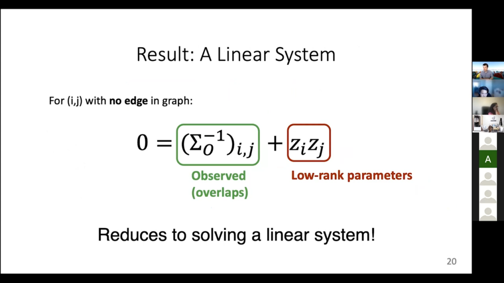
You can decompose this thing into a bunch of equations instead of having matrices, and basically you say “I have these parameters I need to solve for. I have a bunch of equations, I, J, where I know there’s a zero,” which is the left-hand side, and then this gives me a linear system that I can solve. This is a lot of math, but basically all we did here is say, “I can resolve all my accuracy parameters by solving a big matrix equation as long as there’s enough sparsity in this graph,” and this is really what we do in practice. It turns out in simple cases I don’t even need to invert the covariance matrix. But [that] is not an important detail. This can be done for high cardinality. You don’t have to do it for binary. It also even works for data that is continuous. In fact, it works for a lot of stuff in general. That is a fairly general approach, but it is more complicated to solve these equations. I am using all of the information that I have access to.
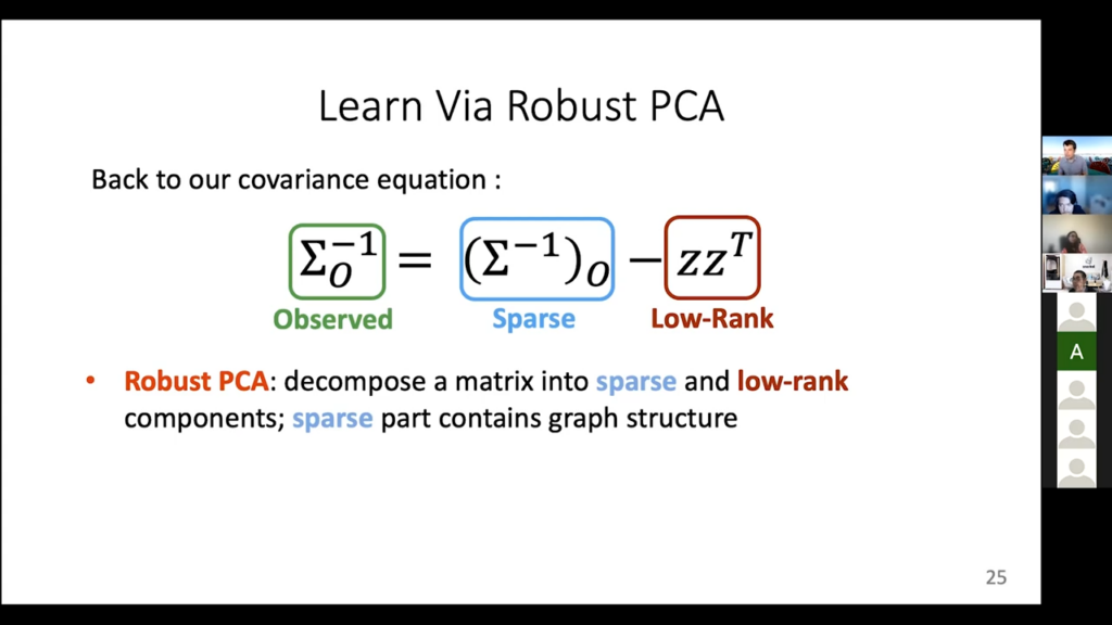
Once you do this you have the full green matrix, which is the entire covariance with all of the accuracy parameters, and the nice thing is you can also prove that this actually works under certain conditions in practice. And one more thing: if you don’t know the dependency structure, so you don’t know who’s coordinating, there is a yet further way of learning it that you would do using this tool called a Robust PCA, that can decompose a matrix into the sum of a sparse and low-rank matrix. I am not going to talk about the details about this thing. It is also incredibly finicky. But we do have this implemented as well, and one of the more advanced label models will use this kind of information that comes from it.
Where to connect with Fred: Twitter | Website.
If you are interested in learning with us, consider joining us at our biweekly ML whiteboard.Stay in touch with Snorkel AI, follow us on Twitter, LinkedIn, Facebook, Youtube, or Instagram, and if you’re interested in joining the Snorkel team, we’re hiring! Please apply on our careers page.

Recommended articles
View all articles

Claude Opus 5: Performance and Error Analysis on Frontier Coding Tasks
Anthropic’s Claude Opus 5 recently debuted as the second model overall on the current Senior SWE-bench leaderboard, behind Fable 5. It also achieves the highest score of any evaluated model on the benchmark’s Bug & Performance Investigation category, reinforcing the rapid progress frontier coding models continue to make on increasingly realistic software engineering tasks. Just as notable, Opus 5 reaches
July 27, 2026
•

Senior SWE-Bench: Evaluating Coding Agents Like Senior Engineers
At our latest Snorkel AI Reading Group, Henry Ehrenberg presented Senior SWE-Bench, an open-source, Harbor-compatible benchmark for evaluating coding agents on realistic, senior-level software engineering work. Its 100 tasks, with 50 public and 50 kept private to mitigate contamination, are sourced from real pull requests across 12 production repositories and cover complex features, migrations, bugs, and performance issues. Senior SWE-Bench
July 16, 2026
•
Snorkel Team

Grok 4.5 Testing Results: How SpaceXAI’s New Model Performs on Real Professional Work
We’ve evaluated Grok 4.5 on Snorkel’s GDPval+ dataset, Snorkel’s expert-created dataset of professional workplace reasoning tasks from across the economy. To compare performance against other frontier models, we ran the evaluation alongside GPT 5.5 and Claude Opus 4.8. Overall, Grok 4.5 demonstrated the strongest overall performance. Dataset GDPval+ is part of the Snorkel Data Series (SDS), Snorkel’s portfolio of expert-curated
July 8, 2026
•

