
Showcasing Liger—a combination of foundation model embeddings to improve weak supervision techniques. Machine learning whiteboard (MLW) open-source series
In this talk, Mayee Chen, a PhD student in Computer Science at Stanford University focuses on her work combining weak supervision and foundation model embeddings that improve two essential aspects of current weak supervision techniques. Check out the full episode here or on our YouTube channel.
Additionally, a lightly edited transcript of the presentation is below.
Motivation
Hi everyone. My name is Mayee and today I’m going to share some recent work. I’d also like to thank Snorkel and Roberto for making this ML Whiteboard talk possible.
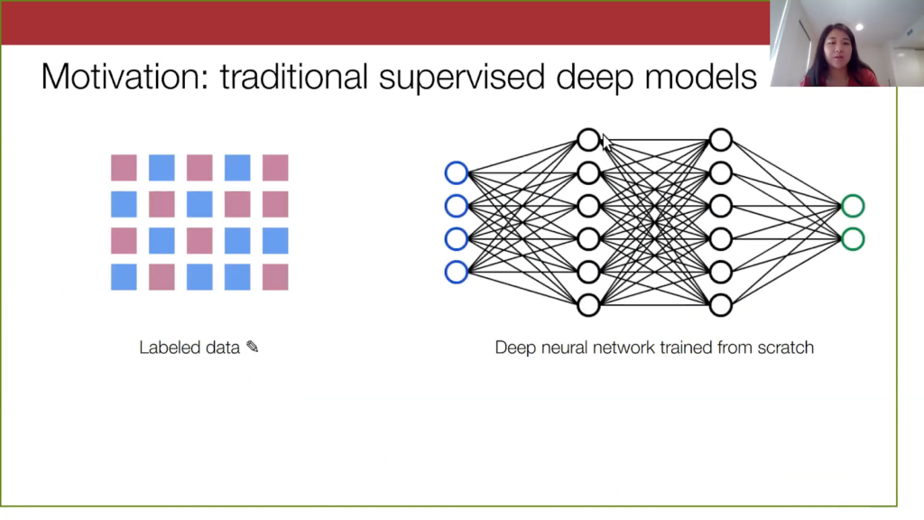
To motivate our work, let’s look at a traditional machine learning setup. We assume that in a supervised learning setting, we typically have a large label data set. Then we train a deep neural network from scratch on it. What is the problem with both of these steps? In practice, acquiring labeled data can be very time-consuming and expensive, and training a deep neural network from scratch is also pretty costly. This makes machine learning less accessible to practitioners who want to use it day-to-day.
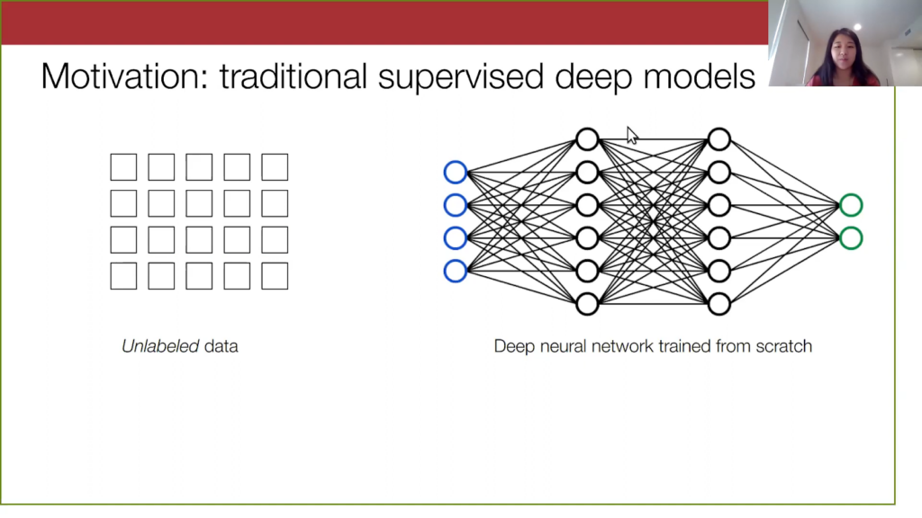
If we start with an unlabeled data set, it takes a long time to label. You might need to hire people to label it, and you also might even need very specialized domain expertise to properly generate highly accurate hand labels. This will slow down the process overall. On the model side, if you want a model that performs sufficiently well, you will need to train for a long time and you’ll need access to, oftentimes, a lot of computing resources. The question here is: how do we make machine learning more accessible to practitioners by relaxing these requirements on both the data side and the model side?
Let’s suppose we start with an unlabeled data set. We can do things here like active learning, semi-supervised learning, or few-shot learning, where we just ask that the user inputs a few labeled samples. Then, the algorithm takes care of the rest.
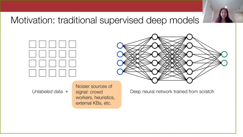
Another angle on this is to take advantage of the fact that there are a lot of noisier sources of supervision that are just lying around for cheap, like crowd workers, user-specified heuristics, knowledge bases. That is exactly where Snorkel comes into play in weak supervision: to figure out how to programmatically label these data sets using noisy sources.
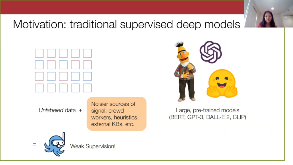
On the model training side, we have also recently seen the rise of these large pre-trained models such as BERT, Open AI’s GPT-3, CLIP, and DALL-E 2 just this week. These models are basically trained on very diverse corpuses of data and are known to generalize well. The nature of machine learning now is that as a practitioner, I can just grab a model off the shelf (e.g. HuggingFace) and then use them for my own task. So, it’s a lot simpler to get these very performant models.
For the rest of the talk I’m going to refer to these models as foundation models, or FMs. When we look at this ML landscape overall, weak supervision has helped make dataset creation a lot easier, because it injects this highly specialized signal for your particular task. On the other hand, foundation models offer very good generalization and thus we can see them as offering very general-purpose information. So perhaps these complementary signals can be jointly exploited.
How do we combine weak supervision and foundation models?
The natural question to ask is: how do we combine weak supervision with these foundation models?
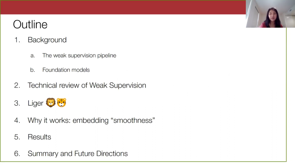
The rest of my talk is as follows: I’ll first provide some background on weak supervision and foundation models. Then I’ll go into a bit of the technical details of weak supervision and discuss our method, Liger, which uses foundation models to address two key challenges in weak supervision. Then I’ll briefly discuss the theoretical properties of foundation model embeddings that allow for our method to work as well as our empirical results, and conclude with a summary and future directions.
Weak supervision pipeline
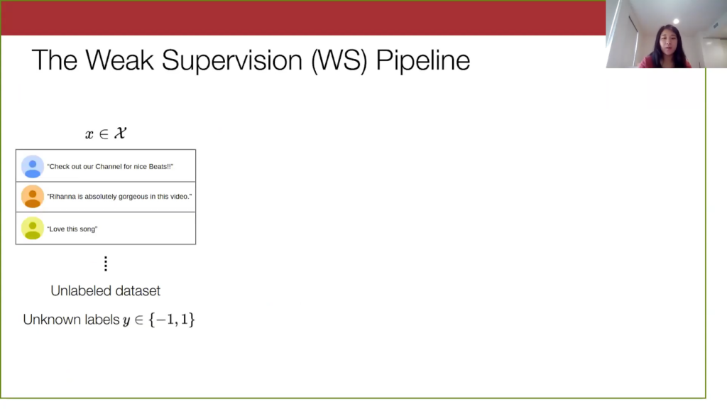
I’ll first describe how the weak supervision pipeline works. We always start with an unlabeled data set with unknown labels that we assume to be binary here, just + or – 1. The example here I have is the spam YouTube data set, which is just a bunch of YouTube comments on some music videos that are either spam or not.
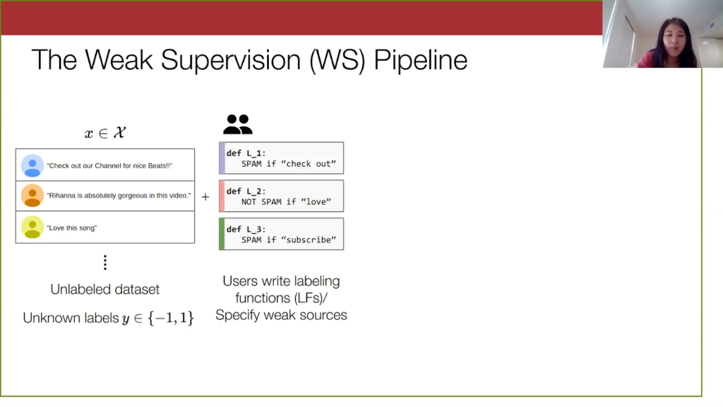
In weak supervision, users will write programmatic labeling functions such as the ones here. I’m going to refer to them interchangeably as weak sources and labeling functions, but you can see how they are noisy heuristics. For instance, if a comment has “check out,” there’s a good chance it’s spam. Another way to think of them is like votes on the true label of a given point.
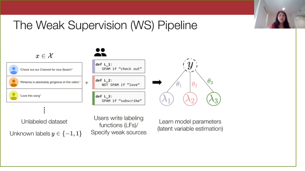
With just these labeling functions, we learn a model over them and the true latent label. I’ll go into a bit more detail about this method later; technically, it’s broadly known as latent variable estimation, but here we are basically constructing a graph depicting the relationship between the labeling functions and the true labels. And we learn these theta parameters here, which you can imagine are these scalar weight parameters corresponding to how accurate a labeling function is and how much you want to value its vote.
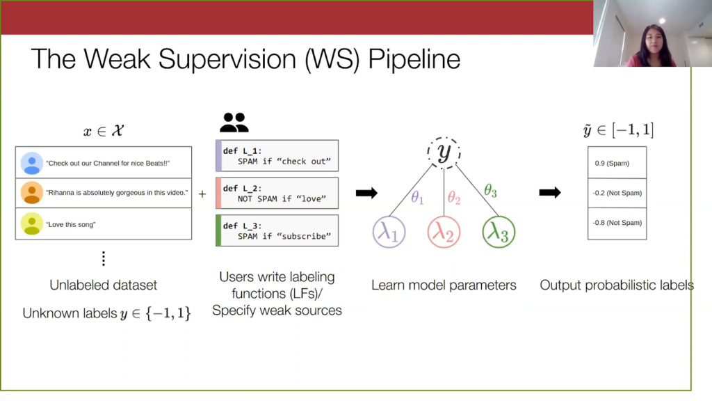
Then finally, we use this learned model to output probabilistic labels. It outputs a score here between -1 and 1, and we just threshold them to get automatic labels on our data set.
For this work, we are mainly focusing on evaluating the quality of the weak supervision pipeline from the unlabeled-dataset step to the probabilistic-label step. But typically, after you get the labels, you can construct your weakly labeled dataset and use it for downstream tasks, such as training a supervised machine learning model.
Foundation models (FMs)
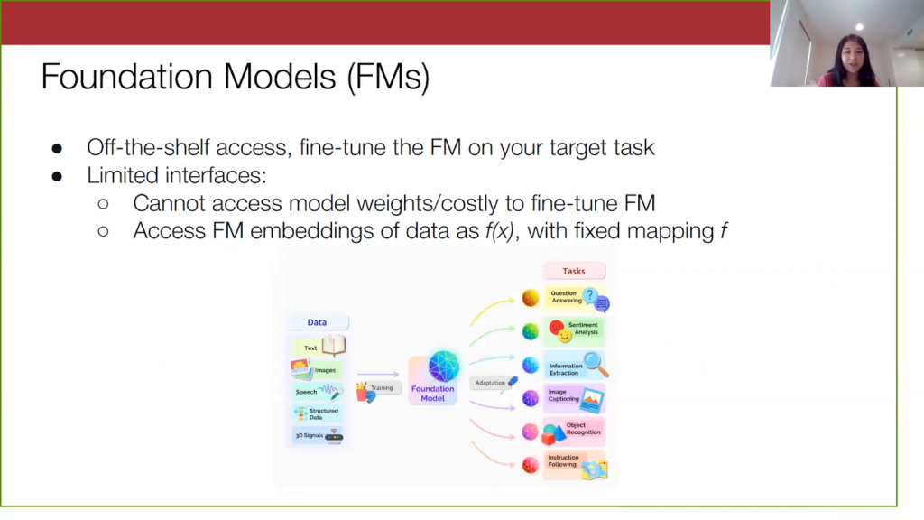
Now let’s turn to the foundation models. As I mentioned before, they are pre-trained on a lot of data and are known to generalize well to many tasks, as shown in this diagram here. To use one like BERT, you import it into your code via Pytorch or some other framework, and then you fine-tune the model on your target task. However, fine-tuning is still technically full training, and so this can be time-consuming and expensive. And if we think practically, we don’t want to continuously retrain models, especially after you deploy it—you just want something very simple and efficient. Furthermore, for a lot of these other foundation models, access to them is limited. Model weights are not typically accessible, and we only really have access to the embeddings of these models via some API. So, a reasonable problem setting is to assume that we are not actually going to be touching the model weights and instead, we access the foundation model via its embeddings. Here I’ve formalized how we’re accessing the foundation model via this f(x), where f is just a mapping from the input space into the embedding space.
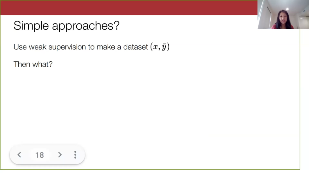
Now that we have established what weak supervision and foundation models are, there are some simple ways to use both of them together. Let’s say we run weak supervision on our unlabeled data set and now we have a weakly labeled data set.
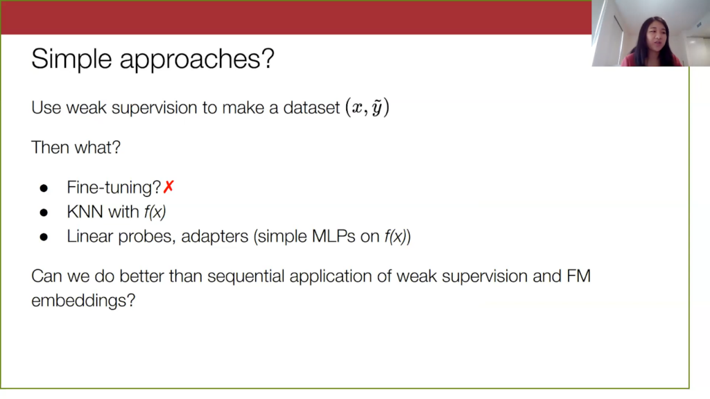
Then we can just sequentially apply the information from foundation models. As I mentioned before, we are unable to do full fine-tuning of the foundation model, but there are other alternatives. For instance, we can just do k-nearest neighbors (KNN) in the embedding space. When we see a new point, our model just gives it the weak label of the point nearest to it in embedding space. We can also fit simple models on top of the embeddings, such as linear probes or adapters, which are just simple multi-layer perceptrons (MLPs) that take in input f(x).
It seems like we ought to be able to do better than just the sequential application of these two concepts, and so what we want to know is: is there a way to use the information from these foundation model embeddings to improve weak supervision in a principled way?
Using foundation models to solve problems in weak supervision
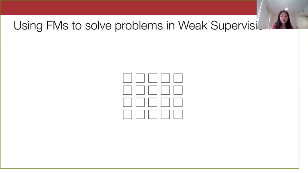
Maybe a way to incorporate foundation models into the weak supervision setting is by identifying current challenges in weak supervision. Here I will give a high level overview of them. When I go into technical detail later, I’ll explain them in more depth.Let’s look at this—a little abstraction of our unlabeled data set we have before.
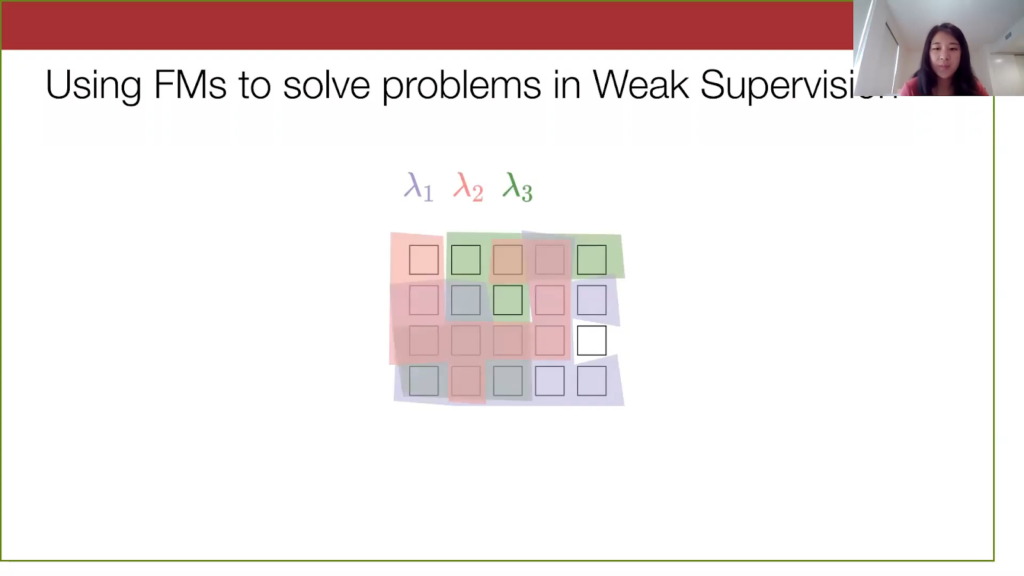
We apply the three labeling functions from the previous spam YouTube example to this data, where the coloring basically shows the data points that each labeling function is applicable on.
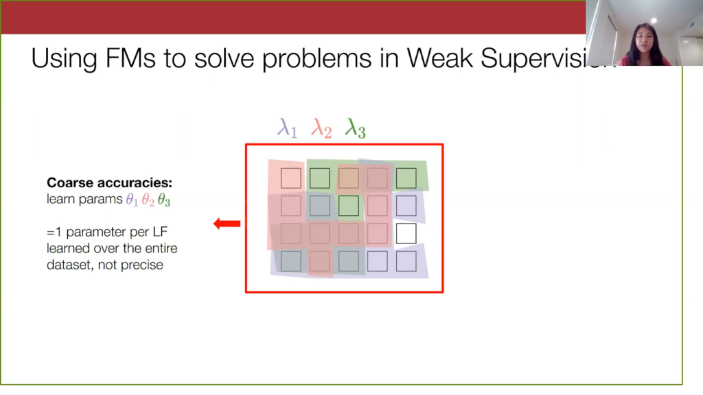
In the current weak supervision setup, we learn a model with parameters describing the accuracy of a labeling function, but we essentially learn one set of parameters over the entire data set. That is, we have one scalar value associated with each labeling function. This assumes that the errors that labeling functions make are completely uniform over the entire data set, but we can perhaps be a bit more fine-grained and precise here to match the subtleties in the dataset.
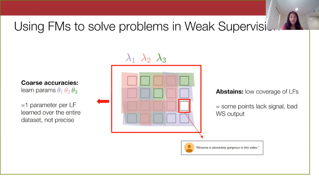
For the second challenge, notice that there’s one white data point that none of the three labeling functions cover, and for points like these we say that the labeling function abstains on them and has low coverage. For this YouTube spam example here, none of the keywords like “checkout,” “love,” “subscribe,” are in this comment. So we don’t really have any information from the labeling functions on it. As a result, when we give the weak supervision model this point, we don’t have votes from the weak sources. Then, the model will be pretty uncertain on this data point and will be more likely to output a wrong label for it.
Before diving in: Weak supervision (WS) 101
To better understand these challenges, we are going to dive into the details of the weak supervision model. This will help us also understand where the foundation model embeddings can help.
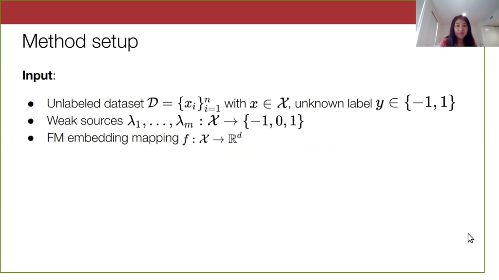
Let’s formalize this setup. We have our three ingredients I mentioned before. We have this unlabeled data set and a bunch of these labeling functions that can either vote +1 or -1—so, spam or not—or they can abstain with a placeholder vote of zero. Then, we have the foundation model embeddings, which we represent as a fixed mapping from the input data to a high dimensional embedding space.
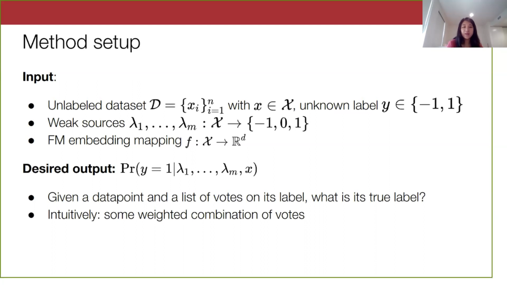
For the output: formally, the output of the algorithm is going to be the probability that our true label is 1, given that we feed into the model our data point and a set of noisy votes on this data point. Intuitively, what we want the algorithm to do is figure out how to combine these noisy votes in the best way. In particular, we want the algorithm to learn the best weighted combination of them, where the weights are essentially our model parameters theta.
Standard weak supervision algorithm
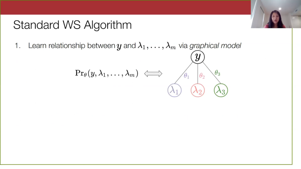
The standard weak supervision algorithm has two steps: parameter learning and inference. The first step is to learn the relationship between the true label and the votes. To do this, we examine the joint distribution over y and the lambdas, and we model this as a probabilistic graphical model that matches the structure on the right-hand side. It’s a very simple structure.
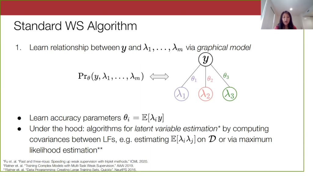
With this model, the theta parameters can be expressed quite intuitively. They are the average rate of agreement between the labeling function output and the true label. You can thus see this theta as a notion of the accuracy of the labeling function. We are going to refer to them as accuracy parameters from here on out.
The first step is to learn these accuracy parameters. The exact procedure can really vary, and there has been a lot of algorithmic work focusing on this. One approach is to do this latent variable estimation. Basically, we compute the covariance matrix between the labeling functions, which are all observable, and we exploit some structure in this matrix to recover the relationship between each labeling function and y. Another one is to simply do maximum likelihood estimation. There are a lot of approaches, and I’m happy to talk about them more.
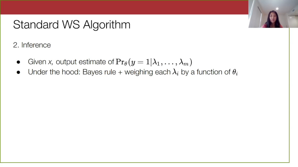
Once we have learned these accuracy parameters, we are mostly done. We just need to write out this formula for how to take the data input and list of votes and convert that into a probabilistic label. It is pretty simple to perform this inference. In the most straightforward case, you would apply Bayes’s Rule to estimate this conditional probability that we want. What ends up happening is you multiply out some simple linear transformations on these accuracy parameters to get your probability.
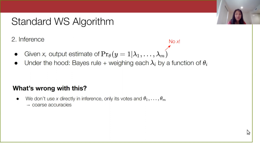
But this overall approach is not perfect, and here I am going to tie back in the two challenges—the coarse grained accuracies and the abstains—that I mentioned earlier. First, note that this probability here does not depend on x. Our model right now is throwing away any potential context we could get from the data point itself, and we are relying only on the information in the labeling function outputs. This is further reflected by how there are only m parameters of our model, which is one per labeling function, to learn over the dataset. This is a more technical explanation of what I meant by coarse, imprecise accuracies.
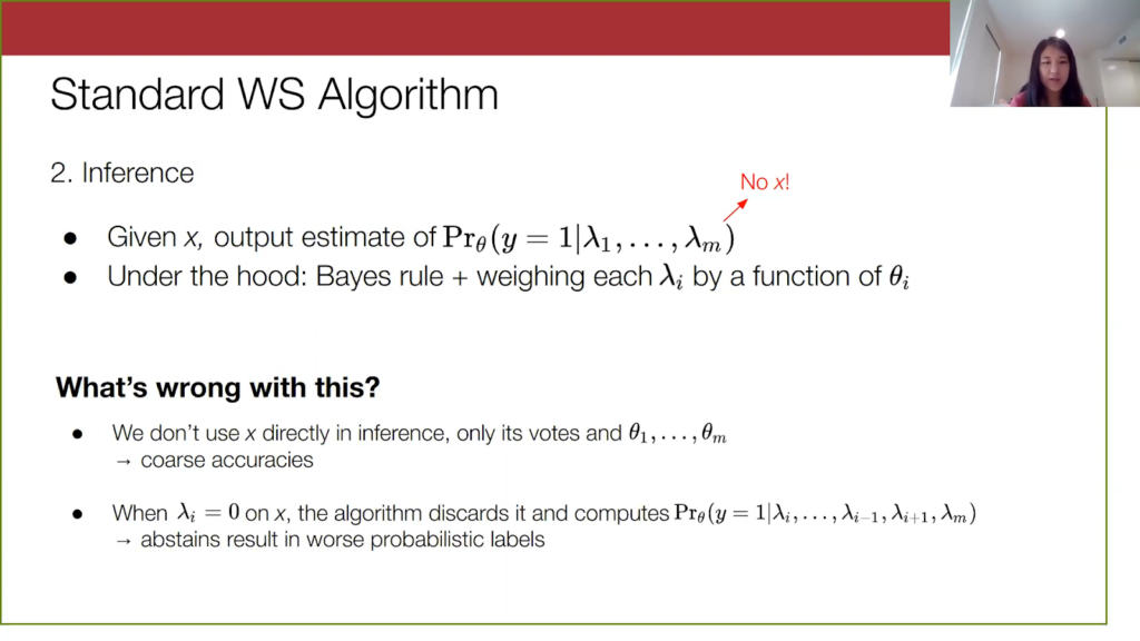
Then the second issue with this graphical model setup is that when a labeling function abstains on a point x—when this lambda_i equals 0 on x—the algorithm will just discard this labeling function’s information away, and we end up computing the conditional probability on all of the other labeling functions’ votes. You can thus imagine an extreme case where all labeling functions vote zero. Then, we are not conditioning on any signal from the labeling functions, and we end up predicting the prior on the probability of y being equal to 1. That’s not good because the model prediction is pretty uninformed.
Liger method: using a combination of foundation model embeddings and weak supervision
Now let’s talk about how foundation models can improve on these two points via our method, Liger.
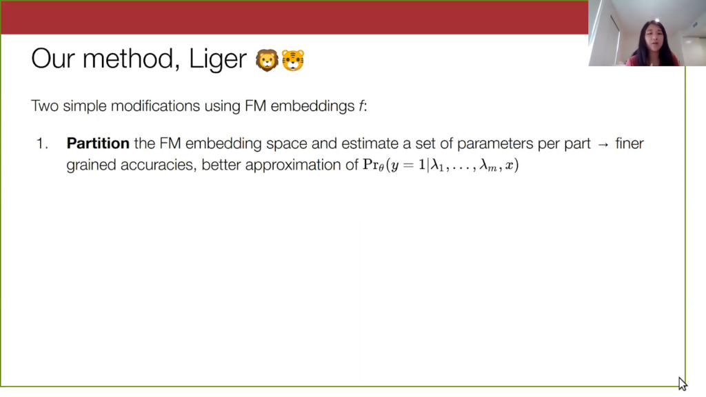
There are two simple modifications. The first modification to the weak supervision approach is to partition the input data in the embedding space and estimate a different set of parameters over each part. This will give us finer-grained accuracy parameters. If we partition into three subsets of data, we now have 3m parameters to describe our model. This will also bring us closer to approximating an output probability that actually takes into account the input data, a probability that is conditional on x.
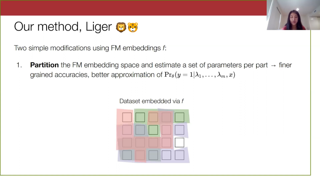
Remember this was our dataset from before with the three labeling functions applied to it, and here I am referring to this dataset mapped into the embedding space of the foundation model.
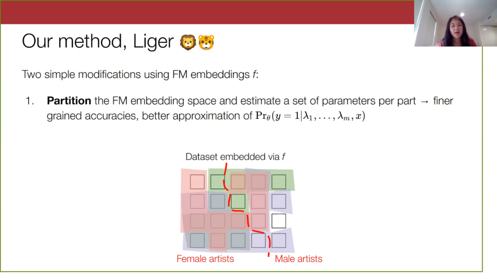
Our method partitions this embedding space, for instance this red line here just for illustration. In these embedding spaces, there might be a natural sort of division in the space between spam comments on music videos done by female artists versus spam comments on music videos and by male artists (this is just an example).
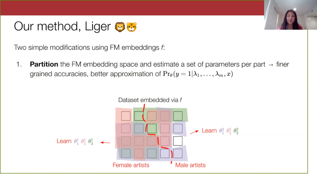
We learn a set of parameters on each of these subgroups, and the hope here is that these parameters will be able to better capture the variation in data.
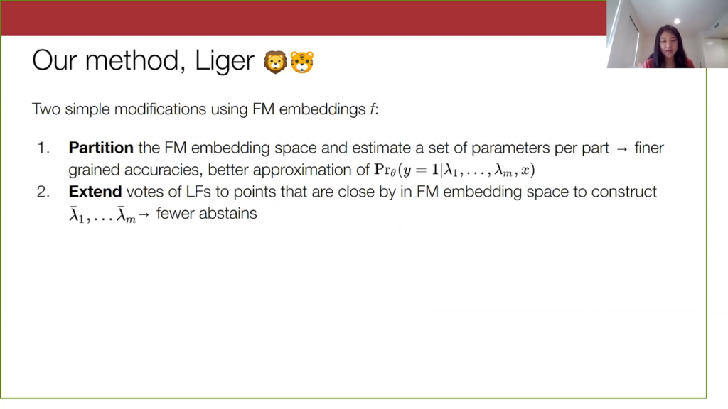
The second thing Liger does is it improves coverage of the labeling functions by extending them in embedding space, in a k-nearest neighbors fashion. So, points that don’t have a vote, but are close to another point that has a vote, will just get the vote of the nearby point propagated to it. This will help reduce the number of abstains and allow for more signal on these points.
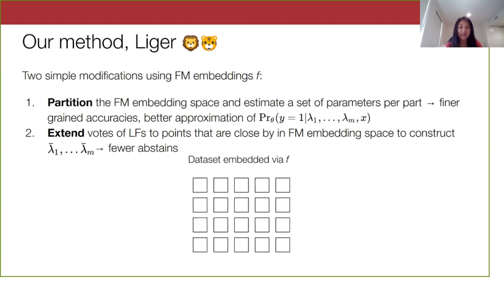
To visualize this, we have our unlabeled dataset from before, and we are going to do a transformation of each labeling function into an extended labeling function by propagating the votes.
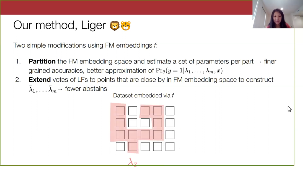

We do this one-by-one, and when we put everything together, our extended labeling functions cover the entire data set—or at least in general cover relatively more of the data set.
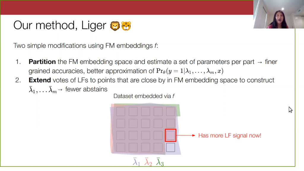
Remember, I identified this data point previously that had no votes on it at all, but now it has a signal from two of the labeling functions. So we will be able to produce a more informed probabilistic output on this sample.
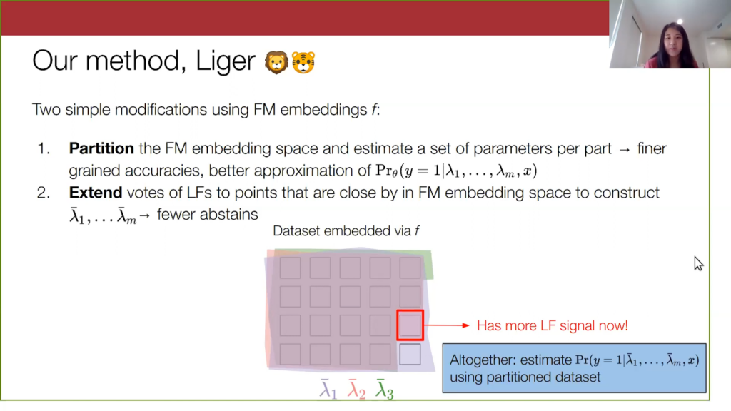
Putting everything together, our method uses these extended labeling functions, which I am referring to at the bottom as these lambda bar. We then learn a model over these lambda bars by using a partitioned data set. That’s it—this is what our method is.
Theory: Why does Liger work?

I will briefly touch on what makes our method work theoretically. Liger relies on this local property of the foundation model embeddings, a notion of smoothness or Lipschitzness of the labels in embedding space. Suppose this diagram below is our embedding space, and let’s look at a particular embedding.
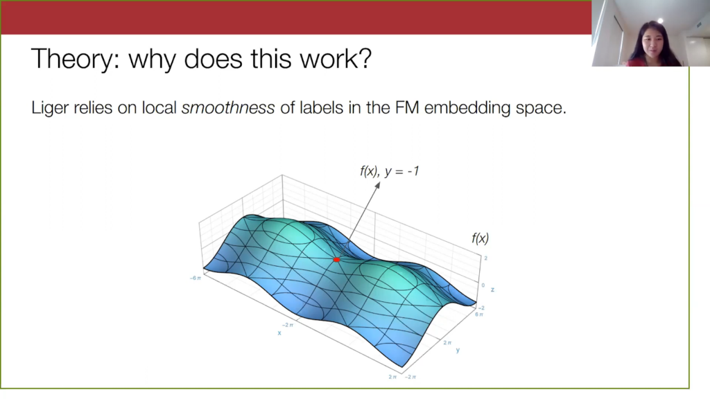
Here is some YouTube comment x embedded by, let’s say, GPT-3, and suppose it’s not a spam comment. Let’s look at points within a certain radius of this original point x.
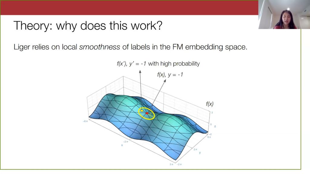
For very “smooth” embeddings, points within a given radius of x will have the same label as x with a high probability. This point x prime here will also not be spam because it is pretty close to x. But on the other hand, as we move farther and farther away from x, we will have less of a guarantee of knowing what the labels of far away points are.
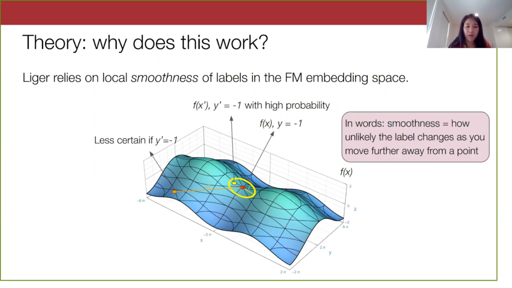
We are less certain if this orange point here is spam or not spam. In general, what I’m describing here is the smoothness of the true label in the foundation embedding space, and smoothness here refers to how unlikely the label will change as you move farther and farther away from a point.

This all makes natural sense when we put it in the context of our method. If we have a very smooth embedding space, you can imagine that when we estimate parameters over this small yellow region, the data distribution within this region is “nice” in some way—it’s not changing significantly. We won’t see anything crazy with how the spam-to-not-spam distribution is changing in this local region. So we can estimate these finer-grained accuracy parameters pretty well.
For the abstains, if we are just extending the labeling function within this small yellow region and the labels are not changing that much in the region, then we would expect that extending a labeling function vote will be correct. Given that a labeling function is already correct on this x, then if we extend that exact same vote to a nearby point (where the y label does not change), our labeling function is still correct. Thus, this extension will provide us with a good signal to work with when the embedding is smooth.
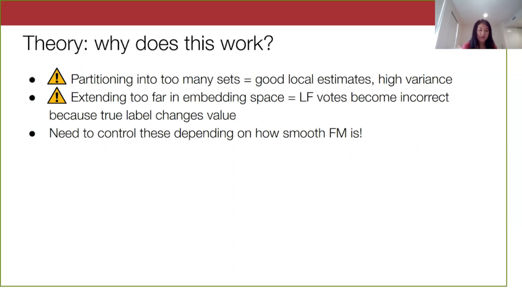
On the other hand, there are things to be careful of here if we go to extremes with the partitioning or extending in our method. If we partition into many sets, the yellow region I described becomes very small. We will end up with very precise estimates of the conditional distribution that we want to output, but we won’t have many points per part to learn over, so our parameters will have high variance. If we extend our labeling functions very far in embedding space, it becomes more and more likely that the true label y will flip as we move farther out. The extended labeling function vote is going to be less reliable as we move farther out. So for these farther out points, it is often better to just have no signal from that labeling function than an incorrect signal from that labeling function. It is very important to control these two hyperparameters—how much you want to partition and how much you want to extend—and we need to control these depending on how good the embedding space is.
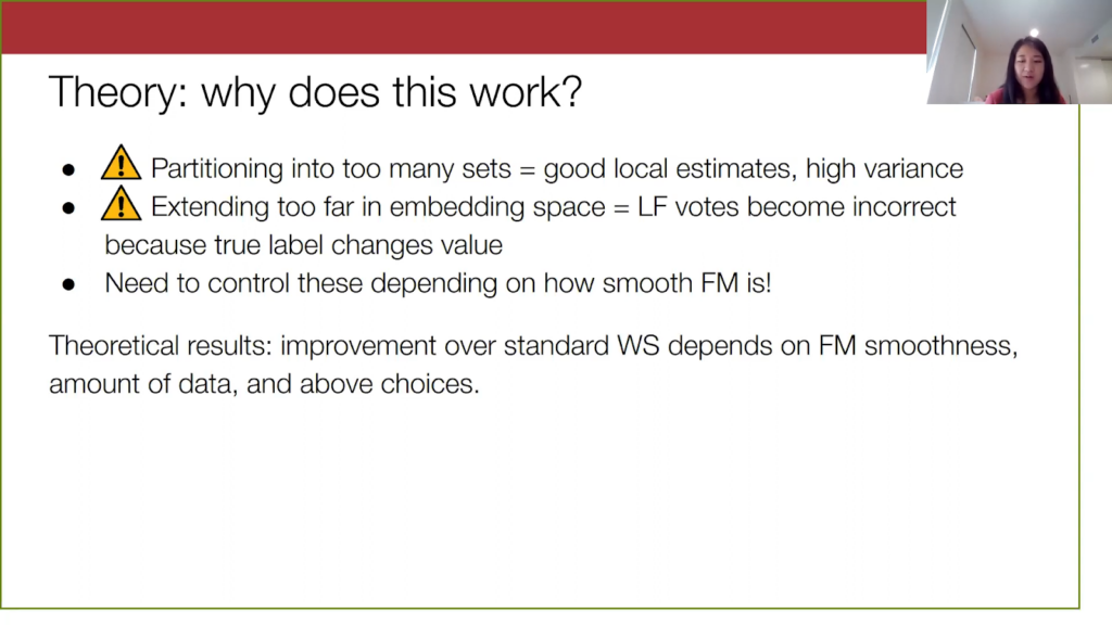
In the theoretical results in our recent paper, we characterize these generalization error bounds, showing how much improvement over the standard weak supervision approach we get, and this depends on the smoothness, how much data we have, and the choice of the two hyperparameters I’ve discussed.
Theoretical results for Liger
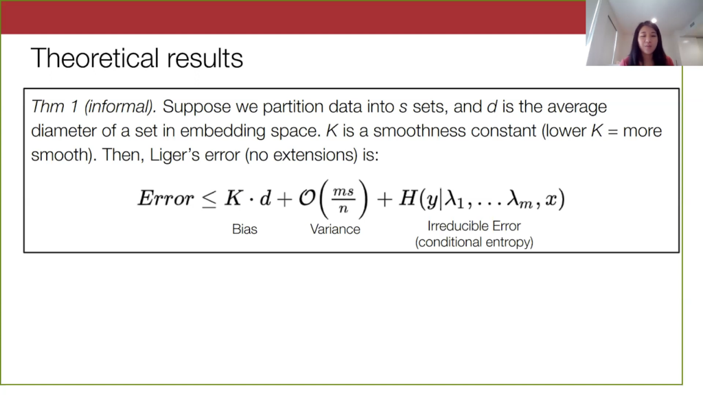
I put in a little bit of the theoretical results that we can go over quickly. For the first result, we are looking at how our method performs when we don’t extend labeling functions. This is just a general error bound for our method. We have a partition into s sets, and each set has an average diameter of d, and k is some smoothness constant. Our result is that we have this bias-variance tradeoff based on the number of partitions. When we look at this bias term and this variance term, increasing the number of partitions s will increase the variance term. But as we continue to partition the data, the diameter of these sets tends to become smaller, so our bias goes down. On the other hand, if we only had one set and did not do any partitioning, the variance will be lower because s is equal to 1. However, our bias will be bigger because this diameter is across the entire embedding space.
Lastly on the right, there is also an irreducible error term. This is the conditional entropy, which is the amount of randomness in y after we observe the data point and the votes on it.
So that was just talking about what the method does and how the partitions display a trade-off.
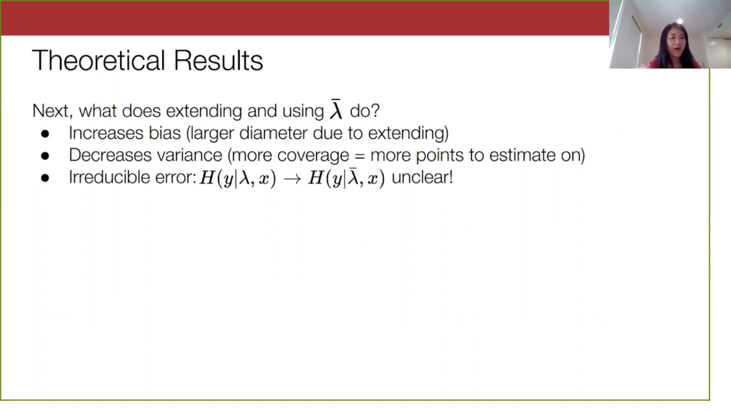
Now we want to know: what does actually extending and using these lambda bars do? Intuitively, it increases bias, because when we extend these labeling functions we increase the diameter of these sets by a bit. We also decrease variance; we improve the coverage of these labeling functions because we have more points to estimate on. So the actual interesting quantity when we do the extension is the irreducible error—how much uncertainty is lambda bar reducing in y versus regular lambda?
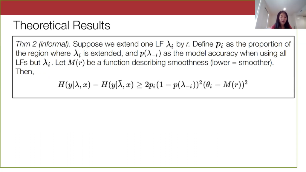
That brings us to our second result, which is a bound on the improvement in irreducible error from using our extended labeling functions versus our not extended labeling functions. There is a bit of notation, but the main things you need to know are that this improvement from using labeling functions depends critically on how much we extend. This extension impacts two quantities. First, pi is what proportion of your data you cover when you extend your labeling function. Then, this M(r) quantity represents how smooth your data is in the embedding space. As you increase the radius by which you’re extending, this M(r) becomes bigger, and this quantity on the right, (thetai – M(r))2 gets smaller. On the other hand, as you increase r, this quantity in the front, pi, will increase.
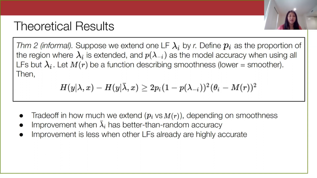
Again, we have this very interesting tradeoff that I intuitively discussed before, where the choice of how much we extend is very important. Two other interesting things are that we will have guaranteed improvement over the non-extended labeling functions as long as our extended labeling function does better than random on average. Second, this middle term p(lambda-i) means that the improvement from extending is going to be less when the other labeling functions are already very accurate.
Real-life Liger results of combining foundation model embeddings and WS
Now for our empirical results: we find that Liger, although very simple, outperforms weak supervision alone, and those simple sequential combinations of weak supervision and foundation models that I mentioned before.
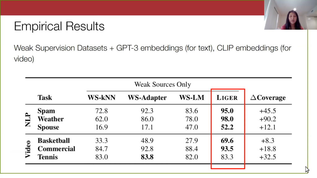
In our experiments, we look at a handful of video and text weak supervision data sets. For the text, we use GPT-3 embeddings, and for video we use CLIP embeddings. The Liger column is highlighted, where we have done a hyperparameter search over the number of partitions and how much we want to extend each labeling function. We outperform WS-LM, which is standard weak supervision, as well as these two other alternatives where we produce a weakly labeled data set and do something simple on it, like k-nearest neighbors or WS-Adapter.
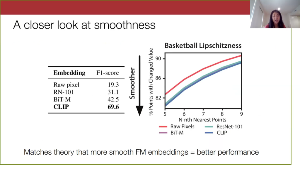
We also want to confirm our theoretical observation that the smoothness of the foundation model embeddings is critical for the performance of our method.For one of the video data sets, we tried our method using some different embeddings. We see that the smoothest embeddings are the CLIP embeddings, because they correspond to the lowest line on the graph here. They also perform the best. On the other hand, the Raw pixel space, Resnet, and BiT are not as smooth and have worse model performance.
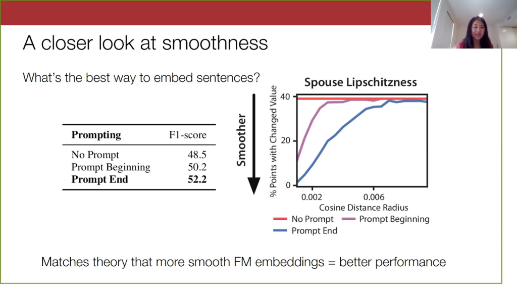
We can also see this on the text data sets. For one of the data sets, spouse (for brief background on spouse, it’s a question data set where you are trying to identify if the two people in the sentence are spouses) we played around with how to embed these sentences and tried three different ways of prompting. We would put this additional text, “Are person x and person y spouses?”, and we tried putting this prompt at the beginning, at the end, or didn’t use the prompt. We find that the smoothness of the embeddings is correlated with the model performance. When we put the prompt at the end, our embeddings were more smooth, and this also did the best. So this matches our theory.
Final thoughts on using foundation model embeddings and WS
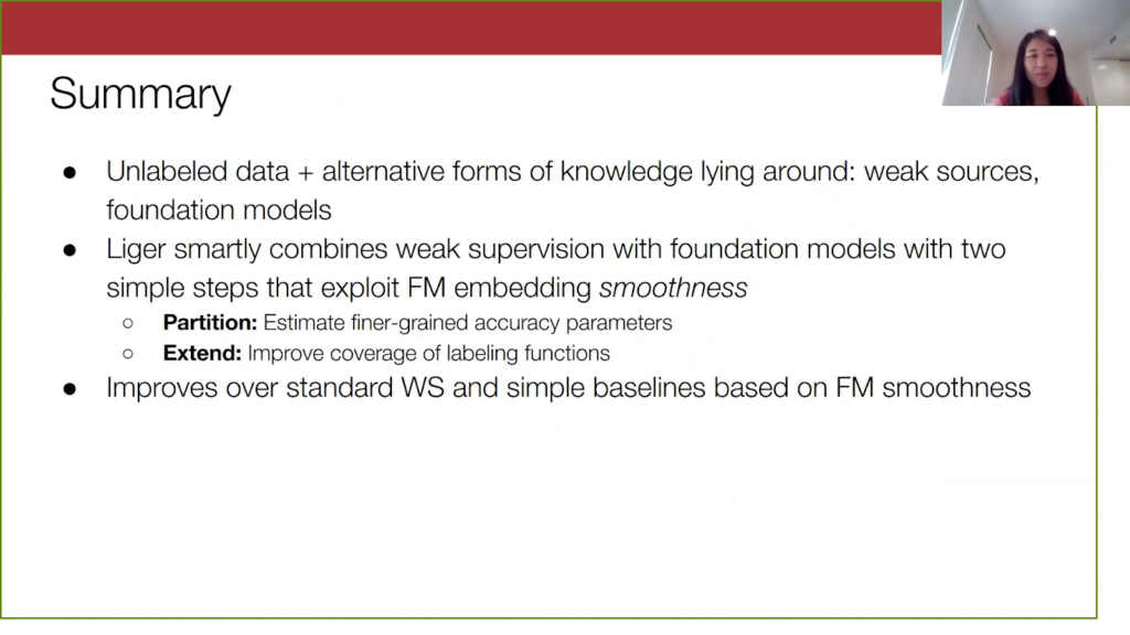
We have reached the end of this talk. To summarize, in machine learning one of the biggest goals is to make deploying models more practical and accessible to everyone. There have been major advances in both directions of the data and the models, in particular by working with these unlabeled data sets and large pre-trained models. Broadly, there has been a lot of work on ways to use these alternative forms of knowledge that are lying around, rather than hand labeling and training from scratch.Our method, Liger, provides a simple way of combining weak supervision with the signal in foundation models, and it consists of two simple steps that exploit the smoothness of label distributions in embedding space. In particular, we partition the data set for richer parameterization, and we extend our labeling functions to improve coverage. We find that this method outperforms standard weak supervision and simple baselines that combine the two concepts, and we empirically confirm that performance is correlated with the theoretical smoothness property.
Future work on foundation model embeddings and weak supervision
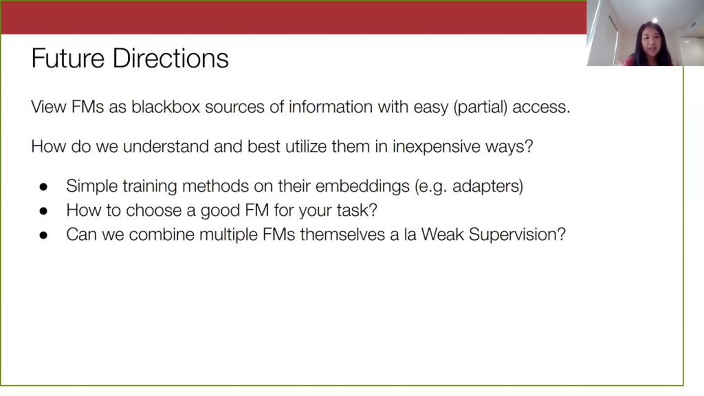
Lastly, I’d like to point out a general exciting future direction. One way we can see these foundation models is as these “black box” sources of information that are easily available to us. Perhaps we don’t have complete access to this model and its trillions of parameters. But I hope that changing the way we interface with these large models can inspire new methods and tools for analyzing them and for how to best utilize these foundation model signals in very cheap and efficient ways.For example, because we often only have access to the embeddings (or it is just simpler and cheaper to work with them) an interesting direction would be to think more about how to train and get meaningful results on just those embeddings, such as using adapters or training “lightweight” smaller models using just these embeddings.Then, since there are more and more of these pre-trained models that are widely available, it becomes more important for us to figure out which one we want to use. A thing I have been wondering is whether you can choose a good foundation model or a good pre-trained model in a very principled way, maybe even by doing some sort of online algorithm for measuring the smoothness or evaluating it quickly. Lastly, as an even more “out there” idea, I am interested in investigating if there’s a way to smartly combine multiple pre-trained models together—potentially even with some sort of weak supervision concept here, since these different representations may have different sorts of information encoded in them. We want to extract as much information as possible from all of them.
That’s the end of my talk. My contact information is above, along with my first co-author Dan’s contact information. Here is the title of our recent work and our link to the paper. Again, I’d like to thank everyone for having me, and I will take any questions.
Q & A
After Mayee’s presentation, there was time for a brief question-and-answer session. It is summarized below.Q: If Liger is built on top of Epoxy, what are its differences from Epoxy?A Liger is basically our little follow-up to Epoxy. The main idea of Epoxy was to focus on those extensions, to fix the problem of abstaining labeling functions. Then in Liger we additionally realized there were other opportunities to exploit the foundation model embedding space. We have that finer-grained accuracy modeling in Liger, where we partition the data set and fit separate sets of parameters, and this allows us to relax the model constraints and get better estimates too.
Q: Can weak supervision problems be solved with boosting? What makes it harder [or] more interesting? Is it that we want to incorporate embeddings from a foundation model?A: With boosting technically it is a setting where we do have labeled data known if I’m correct, and in weak supervision we assume there is no label data at all. The spirit of the method is similar, right? We are just combining these things, but how we learn to combine them is by looking only at these observable sources of information through the labeling functions. I hope that answers the question.
Q: Why should we expect embeddings to be smooth since they are outputs from neural networks?A: If you think about the embedding space…neural networks are not very smooth in that sense, but we are talking about smoothness in terms of the labels. So saying that if we like color and look at this embedding space and your color in which points are spam or not, you’d expect that your spam and not-spam are not going to be just randomly distributed in this embedding space. There should be some sort of signal, and this is a notion of… more broadly, it’s called input consistency, which is an assumption that has been used in these self-supervised or unsupervised algorithms, is that if you have a point with label y, points nearby, with high probability, will also have the same label.
Q: Have you tested using embeddings to train transformers like BERT or others, and do they fall short in comparison to FM models?A: We did in the original version of this…so this is a follow-up to Epoxy. We used BERT embeddings, but that was BERT from 2020, so we haven’t…I don’t think we’ve done these with BERT embeddings. We wanted to try using the newest GPT-3 embeddings. But, yeah, that would be something fun to explore. More of these things, just apply them quickly.
Bio: Mayee Chen is a PhD student in Computer Science at Stanford University, advised by Professor Christopher Ré, focusing on theoretical machine learning. She has published several papers on the theory behind weak supervision at top venues like ICML and AISTATS. More broadly, she is interested in developing theoretical frameworks for incorporating diverse sources of knowledge into machine learning models and evaluating them geometrically. She previously graduated Summa Cum Laude from Princeton University in Operations Research and Financial Engineering, where she received the Ahmet S. Çakmak prize for outstanding thesis research.Where to connect with Mayee: Twitter, Website, Linkedin.Stay in touch with Snorkel AI, follow us on Twitter, LinkedIn, Facebook, Youtube, Instagram, request a demo if you’d like to learn more about Snorkel Flow, and if you’re interested in joining the Snorkel team, we’re hiring! Please apply on our careers page.

Recommended articles
View all articles

Grok 4.5 Testing Results: How SpaceXAI’s New Model Performs on Real Professional Work
We’ve evaluated Grok 4.5 on Snorkel’s GDPval+ dataset, Snorkel’s expert-created dataset of professional workplace reasoning tasks from across the economy. To compare performance against other frontier models, we ran the evaluation alongside GPT 5.5 and Claude Opus 4.8. Overall, Grok 4.5 demonstrated the strongest overall performance. Dataset GDPval+ is part of the Snorkel Data Series (SDS), Snorkel’s portfolio of expert-curated
July 8, 2026
•

Agents’ Last Exam: AI Benchmarking for Real Work
At our latest Snorkel AI Reading Group, Yiyou Sun and David (Xinyang) Han (UC Berkeley, Center for Responsible and Decentralized Intelligence) presented Agents’ Last Exam (ALE) — a benchmark designed to evaluate AI agents on long-horizon, economically valuable, real-world tasks with verifiable outcomes. ALE is a collaboration between Berkeley RDI, Snorkel AI, and 300+ expert contributors across 55 professional subfields. ALE asks a deceptively simple question: can
June 30, 2026
•
Snorkel Team

Continual learning and evaluating how AI agents learn across sequences of tasks
Most agent benchmarks evaluate each task as an independent episode. The agent receives a task, produces an answer, gets scored, and moves on. The next task starts as if the previous one never happened. That setup misses a core requirement for deployed agents. A coding agent, research assistant, data analyst, or workplace assistant should improve as it works across repeated
June 29, 2026
•

