
Constructing labeling functions (LFs) is at the heart of using weak supervision. We often think of these labeling functions as programmatic expressions of domain expertise or heuristics. Indeed, much of the advantage of weak supervision is that we can save time—writing labeling functions and applying them to data at scale is much more efficient compared to hand-labeling huge numbers of training points.
However, sometimes the domain expertise required to construct these labeling functions is itself rare or expensive to acquire. Similarly, there may not be many heuristics readily available to be encoded into labeling functions. What can we do in these cases? More generally, what if we want to augment an existing set of labeling functions with additional ones in order to obtain more signal? Where should we quickly obtain such a set of LFs?
A natural idea is to automatically generate labeling functions. How can we do this?
A simple approach is to acquire a small amount of labeled data and to train tiny models to be used as labeling functions. At first glance, this is counterintuitive. If we already had labeled data, why wouldn’t we just train our end model directly on it? The answer is that we may not have anywhere near enough labeled data to ensure that we train a high-quality model—but we may be able to train small enough models that act as effective labeling functions. Better yet, by creating LFs, all of the advantages of weak supervision, including the machinery of the label model, can be brought to bear.
In this post, we explain at a high level the automatic model-based LF generation process—just one of several possible strategies for labeling function synthesis—and provide some simple takeaways for weak supervision users.
Labeling function generation pipeline
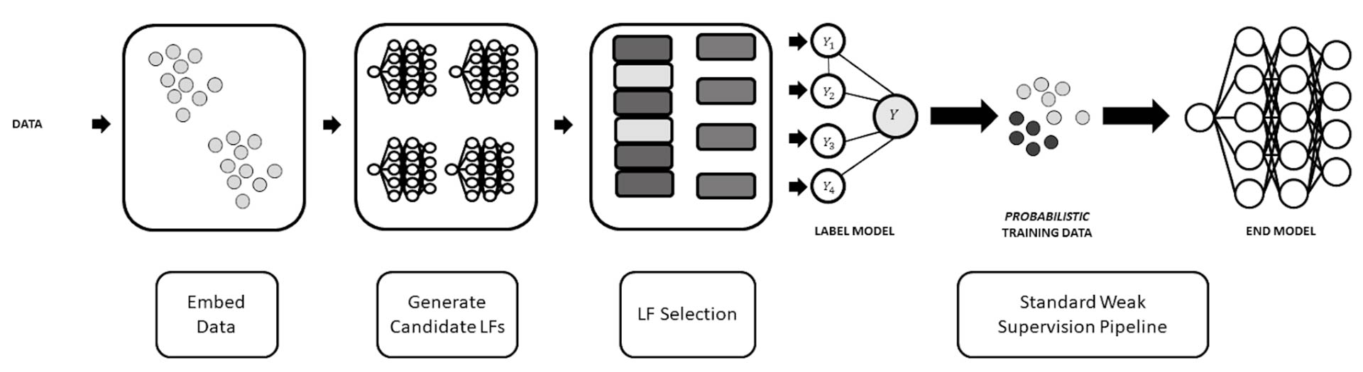 Labeling function generation pipeline. The process interfaces with conventional weak supervision pipelines (right). The three components of automatic LF generation are obtaining representations for the data, generating candidate LFs, and selecting among the candidates.
We can break down the LF generation workflow into three simple steps.
- Embed data: obtain data representations to be used to train labeling functions
- Generate candidate LFs: train a large set of potential LFs based on a diverse set of features and model architectures
- LF selection: choose a subset of the candidate LFs that balance between an important set of metrics.
Below, we explain each step in more detail and provide some simple takeaways.The basic workflow described above was introduced by the Snorkel team on a paper from 2018 for a system called Snuba[1]; much of this post follows the principles described in that paper. The GOGGLES system [2] proposed improvements to handle weak supervision for images. Interactive approaches to further improve LF generation were developed in [3].
Getting your signal
The first step is to obtain representations that we can train our tiny LF models over. In some instances, this simply means the raw features for the unlabeled data. However, these are often not suitable. For example, raw pixel values do not lend themselves to reasonable models, especially when we limit ourselves to very small models. Instead, we can use high-quality representations from pretrained or foundation models. Some examples of the representations we use include
- Raw features,
- Pretrained models like ResNets,
- Foundation models, such as CLIP.
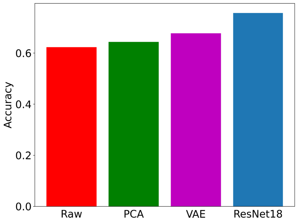
Raw features versus processed features. Raw features for image cases do not lend themselves to workable LFs, but processing features—using PCA, a VAE, or a pretrained ResNet offer better performance. Obtained by running the Snuba algorithm on MNIST with 100 labeled points.
One general takeaway is to obtain representations that capture the salient aspects of the domain. Conveniently, powerful pretrained representations are beneficial and easily available.Choosing the architectures and training the candidates
Our models will necessarily be small—recall that our goal is to obtain complementary signals that capture some aspect of the distribution. We do not seek a large model that can directly be used for prediction. As a result, we use tiny models that are trained over a small number of features. These could include:
- Small decision trees
- Logistic regression models
- Very small MLPs
We do not have to pick among these architectures, but rather generate a large and diverse set of candidates, allowing the next step in our workflow to handle paring down all of the possibilities.How tiny is tiny? One approach, inspired by Snuba, is to consider every combination of one or two features at a time and to train a separate model over them. Another approach we have found useful is to select random combinations of (slightly larger numbers of) features.

Active learning for labeling function training. Without careful choice of the labeled points used for training, the resulting LFs can be highly inaccurate (black separating hyperplane, the outcome from training only on blue points). A few well-chosen points makes a substantial difference in quality (red model is trained on all the data, including red training point).
Another useful takeaway is that the quality of the models is often heavily dependent on the particular configurations of the available labeled data. We have found that using active learning is useful for improved LFs, as shown in the simple illustration above.
Selecting from the candidates
The most interesting aspect of automatic labeling function generation is to select among the candidates. The following desiderata are useful:
- Accuracy: we’d like our chosen labeling functions to be as accurate as possible, since our synthesized labels are ultimately going to be combined (post-label model) and become our labels for training the end model
- Diversity: weak supervision learns from agreements and disagreements in our labeling function outputs. We need a diverse set of LFs to ensure that we have enough potential disagreement
- Coverage: we hope to label as much of our dataset as possible
The selection algorithm needs to balance between these principles. Taking a single one into account at the expense of the others leads to less useful output. For example, prioritizing accuracy leads to identical LFs, and the output labels just reflect this single LF. Worse, to encourage better accuracy, only “easy” points will be labeled—so our coverage will be extremely low. In order to achieve careful balance for these metrics, we can weight the different metrics. To find high-quality weights, we can use standard hyperparameter search tools. This is not required for every new scenario—we have found that it is possible to transfer good choices of weights to similar tasks.We emphasize an additional factor: single the label model operates best with conditionally independent LFs, a fourth criterion for selection is conditional independence.We also note that a lower emphasis on coverage can be mitigated after selection by applying recent ways to inject signal from foundation models for improve coverage, such as in [4].
Comparing auto-LFs to hand-crafted LFs
So far we have discussed the overall idea of automatically creating model-based labeling functions using systems like Snuba, along with some of the key mechanisms that users should take heed of.
At the same time, we might wonder how well such systems work. A full comparison can be found in [1] (and additional comparisons between systems in [2-3]). We showcase a particular example for when these techniques have significant potential: the scenario where human-written labeling functions are particularly noisy. We use the basketball dataset from [5] for a comparison:
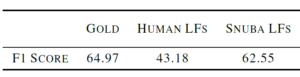
Comparison between fully-supervised model (Gold), using human-written labeling functions from [5], and Snuba-generated LFs using 100 labeled points. In this case, the hand-crafted LFs are noisy and struggle, but Snuba is quite close to fully-supervised.Gold depicts using all labels; Snuba LFs uses the Snuba algorithm on 100 labels. Human LFs refers to the best result from the WRENCH benchmark [6] using the original noisy hand-written labeling functions from [5]. We observe that automatically generated LFs, using just 100 labeled examples, close in on fully-supervised quality, while the noisy human-generated LFs struggle.
Final thoughts
Auto-generating labeling functions is a promising way to construct labeling functions for weak supervision without requiring domain expertise. Such techniques—starting with the Snuba system [1] created by Snorkel team members—have shown significant potential.
How much performance we can obtain from these systems is a function of carefully selecting ingredients. We saw how the quality of the embeddings we use affects the ultimate performance, how we should pick both the right models and datapoints to create candidate LFs, and how to balance different desiderata, like accuracy, diversity, and coverage, when making a final selection of LFs.
Finally, automatically-generated model-based LFs can combine with other Snorkel Flow components, especially foundation model-based labeling functions. We are excited to continue building these combinations.
Bio: Frederic Sala is an Assistant Professor in the Computer Sciences Department at the University of Wisconsin-Madison. Fred’s research studies the foundations of data-driven systems, with a focus on machine learning systems. Previously, he was a postdoctoral researcher in the Stanford CS department associated with the Stanford InfoLab and Stanford DAWN. He received his Ph.D. in electrical engineering from UCLA in December 2016. He is the recipient of the NSF Graduate Research Fellowship, the outstanding Ph.D. dissertation award from the UCLA Department of Electrical Engineering, and the Edward K. Rice Outstanding Masters Student Award from the UCLA Henry Samueli School of Engineering & Applied Science. He received a B.S.E. degree in Electrical Engineering from the University of Michigan, Ann Arbor.
Stay in touch with Snorkel AI, follow us on Twitter, LinkedIn, Youtube, and if you’re interested in joining the Snorkel team, we’re hiring! Please apply on our careers page.
References
[1] P. Varma and C. Ré. “Snuba: automating weak supervision to label training data”. VLDB ‘18.
[2] N. Das et al. “GOGGLES: Automatic image labeling with affinity coding”. SIGMOD ’20. 2020.
[3] B. Boecking, W. Neiswanger , E. P. Xing, and A. Dubrawski, “Interactive weak supervision: Learning useful heuristics for data labeling”. ICLR 2021.
[4] M. Chen, D. Fu, D. Adila, M. Zhang, F. Sala, K. Fatahalian, and C. Ré. “Shoring Up the Foundations: Fusing Model Embeddings and Weak Supervision”. UAI 2022.
[5] Daniel Y. Fu, M. Chen, F. Sala, S. Hooper, K. Fatahalian, and C. Ré, “Fast and Three-rious: Speeding Up Weak Supervision with Triplet Methods”. ICML 2020.
[6] J. Zhang, Y. Yu, Y. Li, Y. Wang, Y. Yang, M. Yang, and A. Ratner, “WRENCH: A Comprehensive Benchmark for Weak Supervision”. NeurIPS 2021.

Fred Sala
Chief Scientist
Frederic Sala is Chief Scientist at Snorkel AI and an assistant professor in the Computer Sciences Department at the University of Wisconsin-Madison. His research studies the fundamentals of data-driven systems and machine learning, with a focus on data-centric AI, foundation models, and automated machine learning. He and his group received the 2024 DARPA Young Faculty Award, a best student paper runner-up award at UAI ’22, the outstanding Ph.D. dissertation award from the UCLA Department of Electrical Engineering, the NSF Graduate Research Fellowship.
Recommended articles
View all articles

Claude Opus 5: Performance and Error Analysis on Frontier Coding Tasks
Anthropic’s Claude Opus 5 recently debuted as the second model overall on the current Senior SWE-bench leaderboard, behind Fable 5. It also achieves the highest score of any evaluated model on the benchmark’s Bug & Performance Investigation category, reinforcing the rapid progress frontier coding models continue to make on increasingly realistic software engineering tasks. Just as notable, Opus 5 reaches
July 27, 2026
•

Senior SWE-Bench: Evaluating Coding Agents Like Senior Engineers
At our latest Snorkel AI Reading Group, Henry Ehrenberg presented Senior SWE-Bench, an open-source, Harbor-compatible benchmark for evaluating coding agents on realistic, senior-level software engineering work. Its 100 tasks, with 50 public and 50 kept private to mitigate contamination, are sourced from real pull requests across 12 production repositories and cover complex features, migrations, bugs, and performance issues. Senior SWE-Bench
July 16, 2026
•
Snorkel Team

Grok 4.5 Testing Results: How SpaceXAI’s New Model Performs on Real Professional Work
We’ve evaluated Grok 4.5 on Snorkel’s GDPval+ dataset, Snorkel’s expert-created dataset of professional workplace reasoning tasks from across the economy. To compare performance against other frontier models, we ran the evaluation alongside GPT 5.5 and Claude Opus 4.8. Overall, Grok 4.5 demonstrated the strongest overall performance. Dataset GDPval+ is part of the Snorkel Data Series (SDS), Snorkel’s portfolio of expert-curated
July 8, 2026
•

