
A primer on active learning presented by Josh McGrath. Machine learning whiteboard (MLW) open-source series
This video defines active learning, explores variants and design decisions made within active learning pipelines, and compares it to related methods. It contains references to some seminal papers in machine learning that we find instructive. Check out the full video below or on Youtube.
Additionally, a lightly edited transcript of the presentation is below.
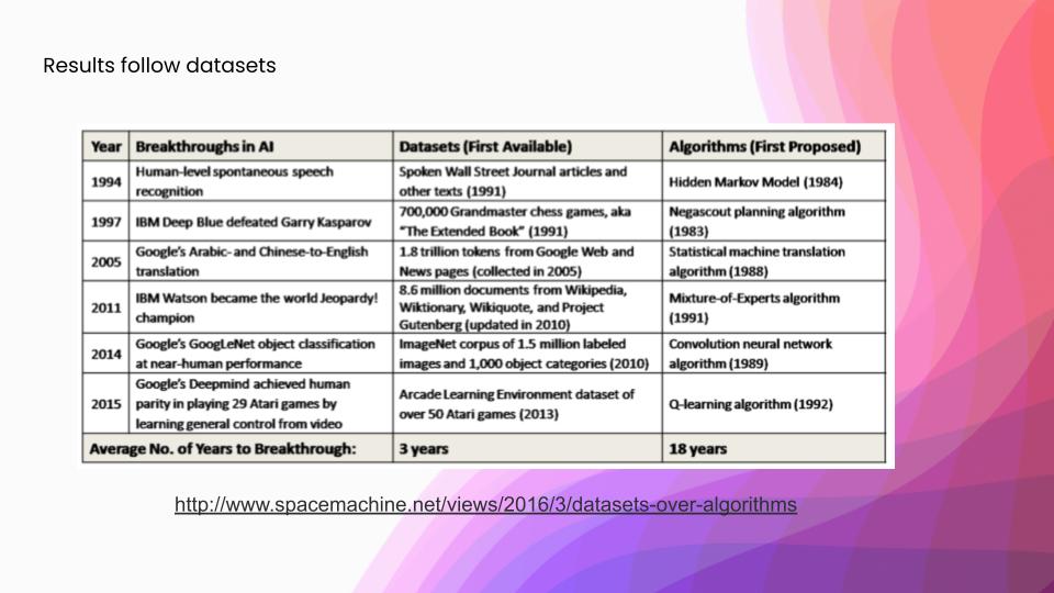
Before we get into active learning specifically, I want to ground the discussion on what is important in building some of these machine-learning systems. We frequently hear a lot about new models crushing a benchmark, however, a lot of that benchmark-crushing is followed a lot more closely by ever better training sets. In this table, you can see some landmark ML benchmarks that have been achieved, and you can see that they’ve been much more closely followed by those data sets—at three years on average—versus the algorithms that were used in the associated papers. What all this sums up is: why are we not spending more time creating these new data sets? Rather, we are spending more time doing model-centric AI development. The answer is largely that curating a dataset is a much harder task than creating a new model. It is a pretty labor-intensive task, with thousands of person-hours spent to build a data set. For a lot of more complex data sets, which have things like medical data, all of those person-hours are prohibitively expensive.
How to deal with the ML bottleneck: lack of training data?
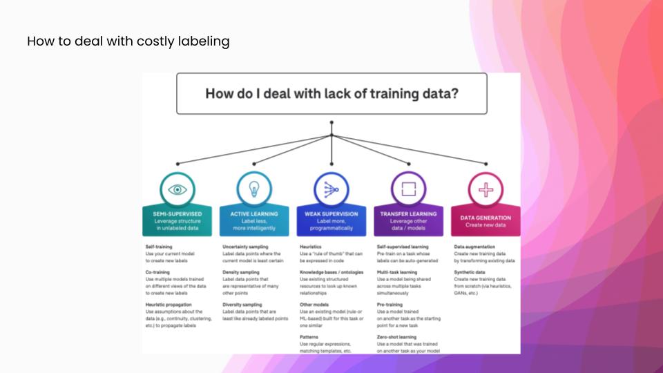
There are a number of different ways to answer this question. Each fits slightly differently into the ML development workflow, and so I’ll just talk at a high level about some of these different answers to it. In semi-supervised learning, we leverage some sort of structure in the data to infer new labels automatically in the data set, after we start with a little bit of ground truth. In active learning, which is what we are going to talk about today, we approximate the informativeness of each example before labeling. Rather than getting automatic labels, we try to have higher impact manual labeling. Weak supervision, which we are big fans of here at Snorkel, is a framework for encoding higher-level sources of supervision as signals, and then integrating all of those into a probabilistic model that can then generate large training sets of somewhat noisier labels. And in transfer learning, we leverage other related data sets or models to complete our task. The most famous examples of these are probably the BERT and GPT families of models, which are all pre-trained on enormous web scrapes of English and then you can use them as the representation model for a wide array of downstream tasks. Finally, we could also generate some extra data, either using data augmentation to take our existing label training set and generate new data from it, or generating entirely synthetic data— something like using a GAN or a simulation framework.
Today, we are going to talk just about the active learning answer to that question.
What is active learning?
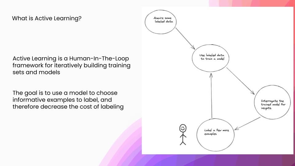
Drilling down on what exactly is active learning: active learning is a human-in-the-loop framework for iteratively building training sets and models. The goal here is to use a model to choose informative examples to label and therefore decrease the overall cost of labeling, because you have to label fewer examples. In this loop, we will acquire some labeled data and we will use that to train a model. We are going to interrogate that model for some insights about what new examples would be useful, which we are then going to send over to a human to label.
Designing active learning pipelines
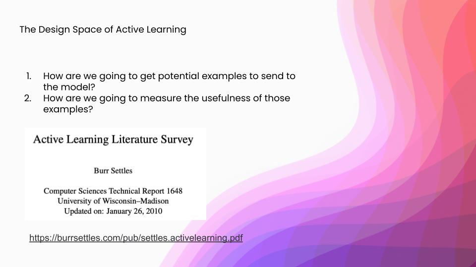
What are some of the design choices that we have within building some of these active learning pipelines? There are two major questions. One is: how are we going to get potential examples to send to the model after being labeled? And two is: how are we going to measure and rank the usefulness of those examples? Now, a lot of the information that I’m about to go comes from this active learning literature survey by Burr Settles. I would say it is one of the better overviews of active learning. If you want to get a sort of technical “deep dive,” that is more in-depth than this, I would recommend starting here.
How to get examples for active learning?
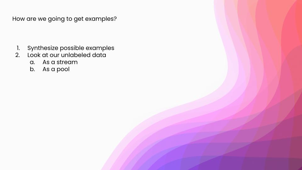
On to that first question: how are you going to get examples? There are two broad families of example-generation for active learning. One is synthesizing possible examples that are unlabeled that we are then going to send to label. The other is when we have some sort of natural distribution from our original problem, and we could view those as a stream or as a pool and each one of those has some sort of different impact on the downstream task.
De novo generation
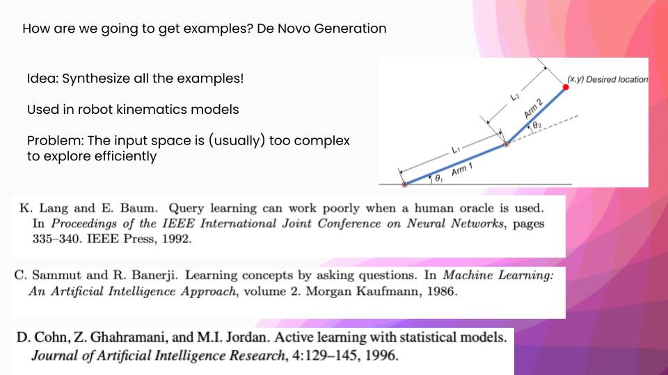
First, let’s get into synthetically generated examples. This is also called “de novo generation.” One of the tasks that this is actually still used today is robotic kinematics. You have amounts of power that you can send to different motors, and you are at two current angles and you have a goal state. Given two angles and some power states, we want to get to a desired (x, y) location. What they will actually do is look at all the possible examples that they could send the model on the circle of the two thetas and then they will see which points the model is the most confused on. It works really well for those sorts of problems. However, if you look at that first paper I mentioned, query learning can work poorly when a human oracle is used. They actually were trying to do a text categorization task using this sort of de novo generation, but they realized that the space of possible English sentences doesn’t have this underlying structure that makes it easy to search for the best examples to send the model. They had to use some other techniques in order to get new examples to send to the model, and that was where we saw some of the first examples of stream and pool sampling, which come from your natural data distribution.
Stream sampling
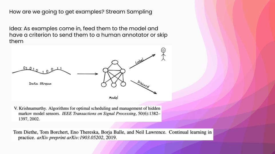
The first of these is stream sampling. The idea is, as examples come in, feed them to the model and have a criterion on whether or not you are going to send those to a human annotator or just skip them. This is still commonly used in sensor setups where there is a natural stream structure to your data. It is not that frequently used in a lot of other problem domains anymore. However, it has a thematic successor in things that have a lot of distribution shifts. For example, the paper, “Continual Learning in Practice”—an Amazon paper presented at NeurIPS 2019, talks about how they have all these data distribution shifts around how people search on their website, and so they have to retrain their models. There are a lot of thematic similarities in these stream-active learning setups, and then retraining pipelines.
Pool sampling
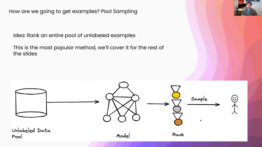
By far the most popular setup for active learning is something called pool sampling. In this what we are going to do is get an entire pool of unlabeled data, and we are going to run our model on all of them and we are going to produce a ranking of all of these different points, in terms of their informativeness to the model. (And I will get into what that means a little bit later.) Then we will either sample or select some of the examples from this ranking and we will send them on to the human annotator. This is by far the easiest because people tend to have these large pools of unlabeled data already, so it is a natural way to formulate the active learning pipeline.
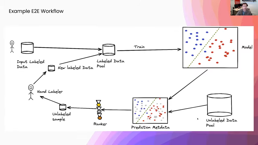
Before I get into some more of how we measure informativeness, I just want to review the high-level workflow. We are going to start with some input hand-labeled data that is going to be labeled by some humans in the beginning, and we are going to use that to train a classifier. Then we are going to apply this trained classifier to an unlabeled pool of data and we are going to collect some sort of prediction metadata of what the model has to say about each one of our data points. We are then going to use this prediction metadata to produce a ranking over all of our different examples in our unlabeled pool and we will use that to select a sample of unlabeled data that we are going to send to hand labelers. We will get some new labeled data that we are then going to add to our label data pool and we will re-enter the training loop from there.
Now, I’m just going to focus on this prediction metadata that we are going to gather, as well as how we are going to rank examples.
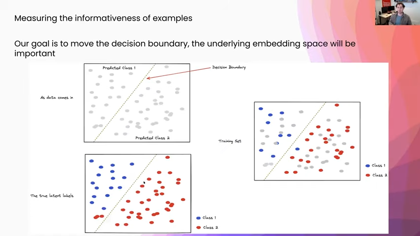
So, informativeness: what does it mean? Our goal is to move the decision boundary, which is this green line in the picture, and so the underlying embedding space is really what we want to be thinking about when we are going to measure informativeness. I want to just talk for a second about what we are looking at here. As data comes in, we just see these gray points. All we are seeing is the input and underneath there is some true latent space, and that is where all the real classes are. You can see in the bottom left here that we have a two-class classification problem and our current model, you can see it is mispredicting things in that bottom left-hand corner. Everything on the right-hand side of the line is class two, the left-hand side is class one. You can see there our current model is misclassifying some things as class one in the bottom left-hand quadrant.
Our goal is basically, as data comes in, and through this upper-left-hand corner we want to generate a training set, which you see on the right, that is a good representation of the true underlying latent space.
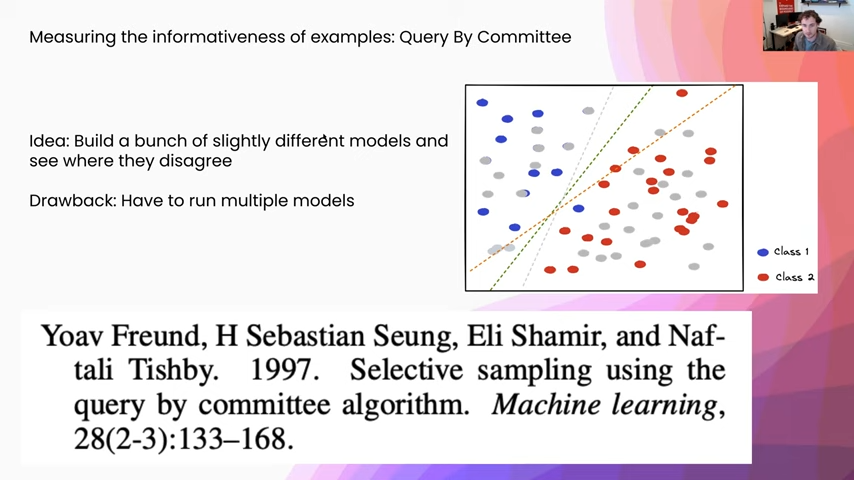
Measuring informativeness, how are we going to do this? One of the possible ways we can do it is something called “query by committee.” We are going to build a bunch of slightly different models and see where they disagree. In this example, you can imagine that we use some different priors or different regularization mechanisms on three different models and we get three different models out. Then we can see where they disagree. One of the drawbacks of this approach is that we have to run multiple models, which I will get into in a second.
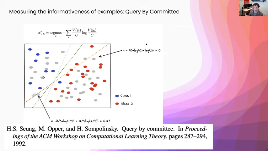
Once we have our different models, how are we going to aggregate their votes together? The most common way to do this is called the vote entropy, and that is saying each one of these models is a voter, and then we are going to take the entropy of the vote distribution afterward. Here you can see I just gave some example calculations. This gray point here, you can see that all three classifiers put it on the right-hand side. There is zero vote entropy there. So we are definitely not going to select that example, we gave it zero weight. Whereas here, in this example in the bottom left quadrant, you can see that two of the examples put it in class one and one model put it as class two. So we get this vote entropy of 0.27, and that way we are going to be much more likely to select examples that are near this decision boundary and that are going to be more informative to our model.
Active sampling
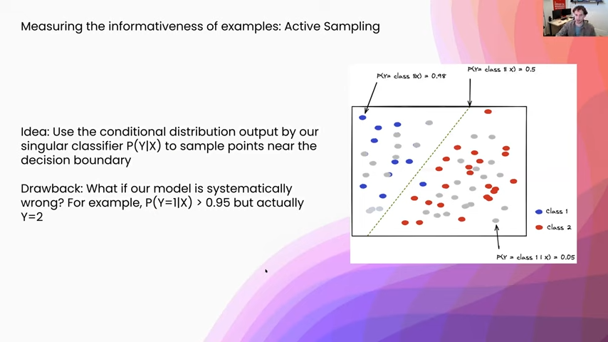
The drawback to that, as I was saying, is that we have to run a bunch of models, which is just a little bit impractical. So one of the other more common things that people do is something called active sampling. What you are doing here is actually leveraging that many of the classifiers we use are not just outputting, say, a single prediction. They are outputting an entire distribution. Specifically, the probability of the class label given some input. We can use that distribution as a proxy for things that are nearer to the decision boundary, or where the model is more confused. So actually that decision boundary is in a two-class classification problem, where we have a 50-50 chance between either class.
One drawback to this approach is that if our model is systematically wrong—for example, it says that something is 95 percent probability one class but it is really incorrect—this is not going to be well captured by an active sampling regime. There is this underlying assumption that our model is what we would call “well-calibrated,” and what that means is if it says you know something is 95 percent probability one class, if it says that for a group of 100 of them you know roughly 95 are going to be actually that class.
Active sampling with uncertainty
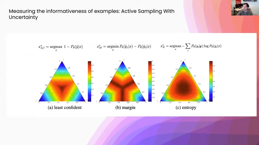
How are we going to take that probability distribution and turn it into a single number that we can rank? The picture you are looking at here are three of the most common measures for turning that probability distribution into a score. Just to give you an idea of what you are looking at, this is a three-class classification problem and you are seeing the probability distribution along these three axes. Right in the center is where everything is probability one-third—you have the uniform distribution. This upper quadrant is where things are most likely class one. In the bottom right-hand, you are seeing class two, and so on. On the left, this point that we are looking over here, you can see the heat map for least confidence scoring, which is basically: it’s going to assign a higher weight to points that the model is least confident on, and where confidence is just the probability of the max probability class. It’s the most interpretable just because it is directly what my model is least confident about.
However, some of these other measures are a little bit more useful. For example, to the right in margin sampling, this is: what is the minimum difference between the two closest classes. The really nice thing about this is, if you have two class confusion in a multiclass problem it is still going to assign a high weight to those examples that are potentially one of two classes. Whereas you can see the others assign a lot more weight closer to the uniform distribution where it is confused between all classes, not just two specific points. So you get quite a bit more diversity with one of these margin sampling schemes, it is quite a bit more robust.
One of the most popular metrics is called entropy, which you see on the right. I like to think of it normally as a generalization of the least confident metric. Whereas the least confident metric just uses a single number to talk about how confident the classifier is, the entropy is actually making one statistic out of the entirety of the distribution. You get a smoother sampling over the decision boundary. Really, its interpretation is an information-theoretic measure that basically says: what would the model be the most surprised to see? Or, what is it having the most trouble encoding? Because of that, it makes a very good metric to use for some of these active learning problems.
Active sampling with information density
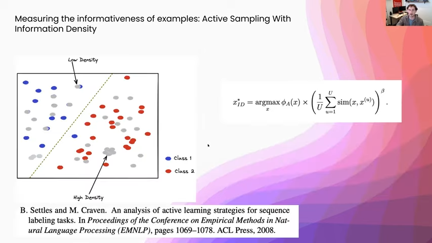
Now, there are some other ways to measure usefulness other than just directly looking at the decision boundary. One of the most popular ones within that is information density. You can think of this as core-set selection, where you are trying to choose a couple of points that represent most of the data set at once. The way that people would measure the information density of something is they would take a representation model—you can imagine taking off the classification head of a neural network or something, or using some sort of pretrained embedding—and using that as a similarity function and then assigning weights to your different points by looking at how many other points they are close to.
Those are just some different ways of assigning scores to each one of our different points. Once we have done that, we have two other choices. One is how many of these examples should we send to the users? And the second is how should we actually select the examples, given these scores?
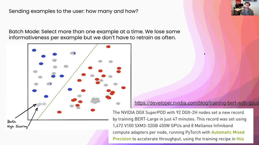
How many should we send? Optimally we should send one example at a time, because we only know what for the current model is going to be the most informative, and if we add a new point to the training set we run into this problem where we can send two points that are too close together, so that way they both essentially carry the same information content. In this example, which you can see in the bottom left-hand corner, both of these two examples are going to be both unlabeled and really high scoring. But if we add just one of them to the training set, we are going to move the decision boundary approximately the same amount. The problem, however, is it takes so long to retrain one of these models that just adding one example at a time is impractical for any sort of realistic setup. I just linked an article down here that talks about just how expensive some of these pipelines are. So using over 1,400 GPUs, it still takes roughly 40 minutes to train some of these BERT models. It’s not really going to be an interactive loop, but we have a human in it, so we are going to need a lower time SLA to use this reasonably.
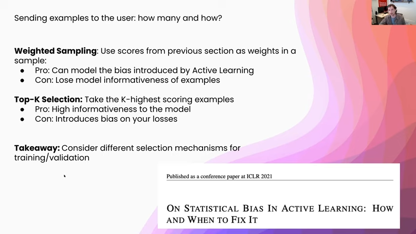
Once we have decided how many and how large we are going to make our batch. We want to choose, given these scores that we got from something like the entropy or the margin scoring that we were just talking about: how are we going to take those scores in and turn them into a selection mechanism? One of those is weighted sampling and the other is top-case selection.
In weighted sampling, we use these scores from the previous section as weights in a weighted sampling scheme. The “pro” of this is we can model the bias introduced by active learning. Normally, when we are talking about theoretical guarantees for an active learning model, or even for just estimating the accuracy of an active learning model, there is this underlying assumption that we drew examples from the distribution uniformly at random. When we use a sampling scheme, we can at least model how much bias we are injecting into the training process or into the accuracy estimation.
The “con” is, that we lose model informativeness of these examples because we spent all of this time selecting the most informative examples with our scoring mechanism and now we are just going to use them as weights, so we are only going to get the most informative examples with some probability. The way to address that is, instead, to do top-k selection, where we grab all of our scores and we just take the high-k-scoring examples. The “pro” of this is that we get high informativeness to the model because we are specifically taking how informative do we think this example is going to be and using that directly to generate the batch that we are going to send to hand labelers. The “con” is it introduces bias, either into your losses or into your accuracy estimation, and so we want to be careful where we are using this as the key takeaway. If you are using it on your training set you can still get good accuracy estimation by choosing a validation set uniformly at random. If you are interested in learning about how some bias can get inserted into active learning pipelines by doing weighted sampling or top case selection, I would highly recommend taking a look at the ICLR paper that I have linked here.
Alright, now before we get into some empirical evaluation, I just want to review exactly what this workflow is after we have gone over some of the examples.
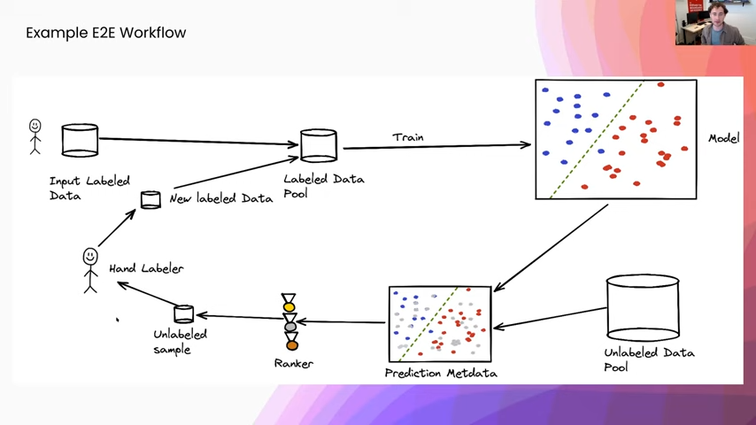
We started with some amount of hand-labeled data that we just selected uniformly at random, and then we started our training loop and we got a first model. We took our unlabeled pool of data and we produced some prediction metadata. In the case that we just talked about earlier, those are mainly two things. One is the probability distribution output by our classifier, and two is where each point was in the embedding space, so that way we can compute things like the uncertainty measures as well as information density. After that we sent those to some sort of ranking mechanism, and that was either top-case selection or weighted sampling, as we were just talking about. After we have done either one of those, we will have this unlabeled sample of data that we are then going to send to hand labelers. They are going to give us a little bit more label data that will then add to the label data pool and re-enter our training loop.
How well does active learning work?
The most obvious question is: how well does this work? How much has it reduced the cost of our labeling process? Let’s get right into that.
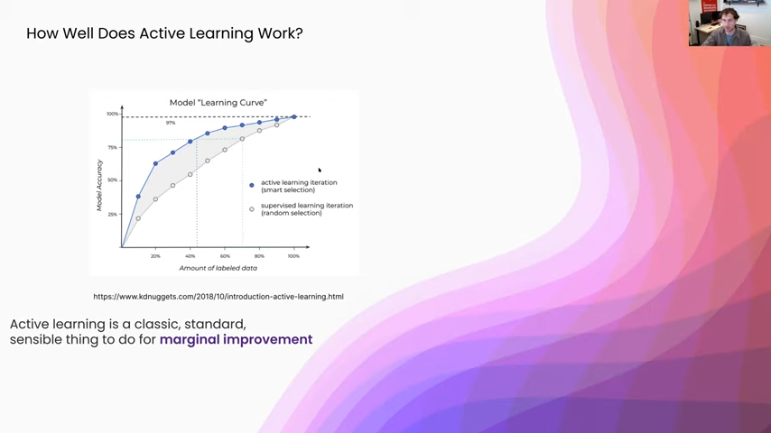
I’m going to go over the empirical results sections from a couple of different papers, but I really liked this KDnuggets graphic, because I think it shows the general trend of how active learning systems tend to perform relative to some random selection baseline. You can see in gray here, this is the random selection baseline. Using some other active learning selection technique, we get the same overall general behavior—as you add more data you are going to scale relatively similarly, but you get the offset just because you are using an active learning selection mechanism. Overall it is a pretty standard and sensible thing to do for a marginal offset of improvement.
Active learning for images
Now let’s get into some of the actual empirical results sections from a couple of different papers.
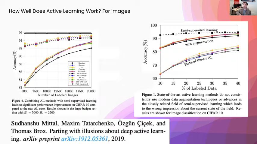
I really like this paper specifically: “Parting with Illusions About Deep Active Learning.” It is a great empirical analysis for a lot of different image data sets, using the same model across a ton of different training techniques. On the left-hand side here, you can see, in black, we have the baseline just as if we selected data points uniformly at random. These colored solid lines—these are different active learning selection setups. You can see in blue, that is the entropy. Yellow is a form of doing lowest-confidence sampling, and then core-set selection, which is similar to information density. You can see that we do get this nice offset, where we were getting a marginal improvement. However, if you look above it, there is a semi-supervised comparison where they are using semi-supervised learning. And then yet again they have one where it is just semi-supervised learning. And then it is semi-supervised learning where they are also adding labels in an active learning setup. You can see that there is a huge offset in performance, where even at the point of 5,000 they are still getting almost 10 percentage points higher in terms of accuracy. And just to review, semi-supervised learning specifically, in this case, was self-training. What you do is start with your small labeled pool of data, you train a model on that, and then once you are done training that model you apply it to an unlabeled pool. Then anytime the model is highly confident in one class, you actually add that with the new inferred label to the training set, and you keep training off of this.
Next, on the right-hand side, you can see yet again a couple of different active learning techniques. Then the other line above is with augmentation. In this case augmentation for a lot of image data sets can be doing things like rotating images and changing color channels. That way, you teach the model about different invariants like a yellow car and a red car that look exactly the same other than color. They are still both cars. Or, if you rotate a car, it still is a car. You can see there again, even if we are getting some improvement from active learning, it is marginal. Whereas, if we use some of these other techniques, like semi-supervised learning and data augmentation, we are getting these much larger increases in statistical performance.
Active learning for entity matching
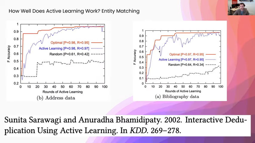
This is for an entity-matching setup, where you have two tables that refer to the same kinds of entities in the world. You can imagine all the people on Wikipedia and then something like, I don’t know, your contact book or something like that, and you want to figure out the mentions of the people in your contact book when they are referring to the same thing as in a Wikipedia article. This is something that active learning works really well on. You can see the baseline black dotted lines on either side of these, versus, in blue, active learning. We are getting a huge increase in statistical performance. Now, actually the reason for that is, in most of these de-duplication setups, all your input to the model is always something like a similarity function. This is actually more like learning a decision threshold than it is learning like a representation. In this case, active learning performs really well.
Now for another empirical results section, for error detection.
Active learning for error detection
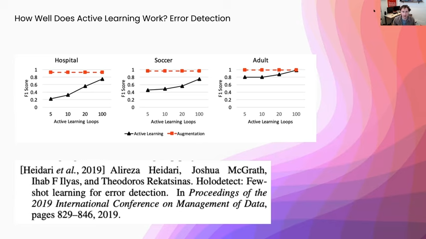
In this paper we were trying to detect errors in tables. So, at the cell level—say this cell is erroneous or not. One of the things that you could do is you can say: well I know that this cell is clean. You can actually inject errors into it and that is a form of data augmentation. You can see on three different data sets we ran just augmentation or we used active learning and we consistently added, I think it was 1 percent or half a percent of the data at each one of the learning loops. You can see here, yet again, with active learning you are still getting a nice boost in between active learning loops. But it does not compare to the efficacy of using data augmentation. In some cases, even when we were giving half of the data set to these models, they still were not performing as well as data augmentation was, just because in a lot of error detection setups there are a lot of class imbalance. So, even using active learning, you might not be able to get enough of your minority class.
Active learning for text data
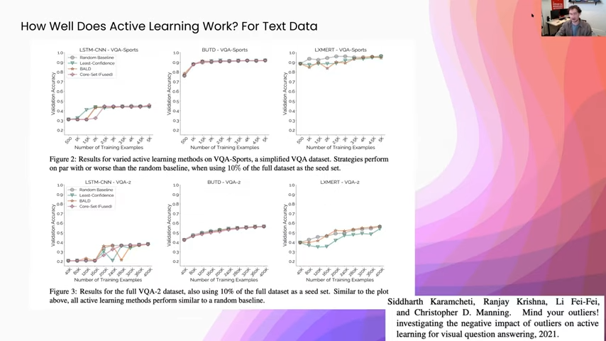
Finally, for some other text categorization tasks, this is specifically visual question answering, and the models that they are using are pre-trained on a lot of English text. One of the things that they found is that active learning can pick out specific outliers if you already have a good representation model. What they realized is, and you can see this especially in the the top set, when you start using active learning it can select only outliers and it actually decreases the performance on downstream tasks, because you are adding really confusing examples to the training set. So I would highly recommend taking a look at this paper: “Mind Your Outliers! Investigating the Negative Impact of Outliers on Active Learning for Visual Question Answering,” because it talks about some of the ways that active learning—when you are using some of these other techniques like pre-training—can actually have a negative impact on your downstream model.
How does active learning compare to weak supervision?
Finally, because we are Snorkel, how does this compare to weak supervision?
This is something that is hard to do, because they don’t have an easy common denominator. In a weak supervision setup, you might not have any labeled data. To start you might not have any label data. You label it using labeling functions. However, since you could be using one labeling function that you write in 30 seconds to generate 10,000 labels, it doesn’t quite make sense to compare them, label to label, because the amount of person-hours that you are spending on that could be totally different. Labeling 10,000 examples in terms of person-hours is a relatively fixed cost if you know how fast your hand labelers can label those. Whereas a single data scientist could write one function to label 10 points or 10,000 or a million, and those are all going to be the same amount of time for the data scientists to write that labeling function.
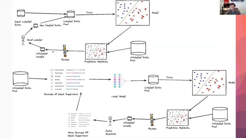
The other piece is we can also modify what is being passed around in these active learning loops to incorporate weak supervision into those. If you look on the top here, this was the original pipeline that we were looking at where we start with some hand-labeled input data and we are basically passing around pieces of data within our active learning loop. However, that is not the only choice that we have. When we are using a weak supervision setup, we can start with our unlabeled pool of data and then our subject matter experts and data scientists can add in a bunch of sources of weak supervision, pass that to a label model, and then get a labeled pool of data. Then we will go through the training loop and collection of prediction metadata and ranking, the same as we were before. But now, instead of sending all of these examples to hand labelers, we can send them to a data scientist to do a round of error analysis or pattern matching on these where they are saying, well, what sources of weak supervision are missing, such that the model is confused on these examples. Then they can go and look for more sources of weak supervision, pass that up to their other set of sources of weak supervision, and restart their label model and training loop as usual in a weak supervision setup.
So we don’t really need to compare these two directly because it is somewhat apples-to-oranges. These two workflows can even really complement each other.
Key takeaways of active learning
- Active learning is the process of using your model to inform what points you should label next in order to best improve that model.
- Its goal is really to make each data point we manually label worth more with respect to the downstream accuracy.
- In terms of performance, it is a marginal improvement over a traditional manual labeling approach.
- There are a lot of other methods, like semi-supervised learning, data augmentation, and weak supervision, that offer a lot larger performance improvements in terms of person-hours to downstream accuracy.
- Finally, we can combine active learning with weak supervision, data augmentation, and semi-supervised learning in order to boost those methods as well.
Bio: Josh McGrath is a software engineer with our Lifecycle team and works on model monitoring, active learning, and error analysis. Previously he was a machine learning engineer at Apple, after Inductiv—an ML startup acquired by Apple.
Where to connect with Josh: Linkedin.
Stay in touch with Snorkel AI, follow us on Twitter, LinkedIn, Facebook, Youtube, or Instagram, and if you’re interested in joining the Snorkel team, we’re hiring! Please apply on our careers page.

Recommended articles
View all articles

Grok 4.5 Testing Results: How SpaceXAI’s New Model Performs on Real Professional Work
We’ve evaluated Grok 4.5 on Snorkel’s GDPval+ dataset, Snorkel’s expert-created dataset of professional workplace reasoning tasks from across the economy. To compare performance against other frontier models, we ran the evaluation alongside GPT 5.5 and Claude Opus 4.8. Overall, Grok 4.5 demonstrated the strongest overall performance. Dataset GDPval+ is part of the Snorkel Data Series (SDS), Snorkel’s portfolio of expert-curated
July 8, 2026
•

Agents’ Last Exam: AI Benchmarking for Real Work
At our latest Snorkel AI Reading Group, Yiyou Sun and David (Xinyang) Han (UC Berkeley, Center for Responsible and Decentralized Intelligence) presented Agents’ Last Exam (ALE) — a benchmark designed to evaluate AI agents on long-horizon, economically valuable, real-world tasks with verifiable outcomes. ALE is a collaboration between Berkeley RDI, Snorkel AI, and 300+ expert contributors across 55 professional subfields. ALE asks a deceptively simple question: can
June 30, 2026
•
Snorkel Team

Continual learning and evaluating how AI agents learn across sequences of tasks
Most agent benchmarks evaluate each task as an independent episode. The agent receives a task, produces an answer, gets scored, and moves on. The next task starts as if the previous one never happened. That setup misses a core requirement for deployed agents. A coding agent, research assistant, data analyst, or workplace assistant should improve as it works across repeated
June 29, 2026
•

