Coactive AI’s CEO: quality beats quantity for data selection

Cody Coleman, CEO and co-founder of Coactive AI gave a presentation entitled “Data Selection for Data-Centric AI: Quality over Quantity” at Snorkel AI’s Future of Data-Centric AI Event in August 2022. The following is a transcript of his presentation, edited lightly for readability.

I’m super excited to chat with you all today. I’m Cody Coleman and I’m really excited to share my research on how careful data selection can make ML development faster, cheaper, and better by focusing on quality rather than quantity.

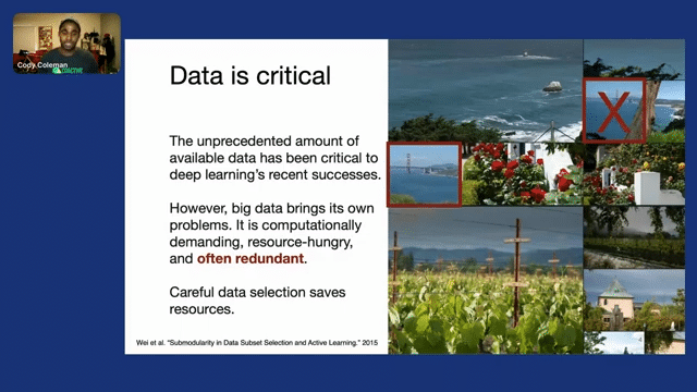
The unprecedented amount of available data has been critical to many of deep learning’s recent successes, but this big data brings its own problems. It’s computationally demanding, resource hungry, and often redundant. So we waste a lot of time, money, and just energy on data points that aren’t actually valuable.

But if we’re instead careful about the data points that we actually choose to label and train on, we can save valuable resources. And just to give a sense of how costly this data can be in getting it wrong, let’s look at speech recognition. Annotation at word level can actually take 10 times longer than the audio clip.

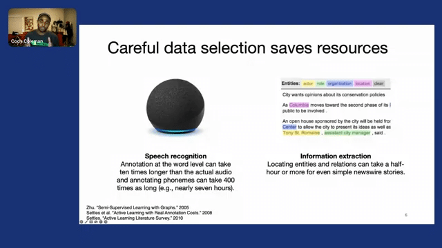
Now, if we do finer-grained annotations, it can take up to 400 times as long. Even for simple tasks like information extraction, locating entities and relations can take a half an hour or more, even for simple news stories. And this is just the time that goes into labeling a single example. Trying to figure out what examples to label is another massive problem where we spend a lot of time and resources actually figuring out how to curate the dataset.

So the key problem here is, how can we efficiently identify the most informative training examples? And we’re in luck. There’s a long history of research, under active learning and core-set selection, which has developed methods that focus specifically on quantifying and identifying the most informative training points.

However, there’s an asterisk here when we think about modern big datasets, but I’ll get to that in a minute. First, what is active learning? The goal of active learning is to select the best examples to improve model quality. And this is done through an iterative process where we start with a large amount of unlabeled data, and then we take a small subset of that, that we label either chosen at random or maybe it’s given to us, and we train a model on that subset.

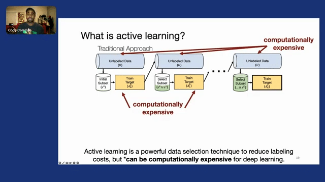
Now this is where the interesting bit happens. We take that model and some selection strategy or criteria to quantify the informativeness of the examples, and we apply that to all of the unlabeled data. And then we can actually select the examples that are the most informative or the most valuable for us to label, we can label those and we can expand our labeled set.

And then we can repeat the process where we train a model, and with this new updated model that uses better data, we can repeat this process of applying it to all of the unlabeled data and selecting the best examples to label until we’ve exhausted some labeling criteria or other constraints, at which point we can train the model one last time on all of the data that we’ve collected so far.

Active learning is a really powerful data selection technique for reducing labeling costs. But when we think about deep learning and modern data workloads, it can be computationally expensive. For example, if we think about this iterative process, retraining a deep learning model after every single step or every iteration can be extremely expensive, which limits how many iterations we can do, or the frequency with which we can do those iterations. And then when we think about modern datasets with millions or billions, potentially, of unlabeled examples, actually scanning over all of the unlabeled data can be a massive computational bottleneck. So, today I wanna talk about two pieces of research that address these computational bottlenecks and constraints.

First, “Selection via Proxy,” which appeared in ICLR 2020. I was super fortunate to work with amazing researchers from Stanford on this. And then second we’ll talk about “Similarity Search for Efficient Active Learning and Search of Rare Concepts,” which I had the pleasure of working on with folks from The University of Wisconsin Madison, as well as Facebook. And this work appeared in AAAI 2022.

Starting with selection via proxy–and going back to this kind of setup that we discussed–selection via proxy tries to address the computational expense that’s associated with training these large deep learning models at every iteration. Now the key insight that we exploit in selection via proxy is that small models can provide a very useful signal for selecting data points. So here in this plot, we actually took a variety of model architectures and sizes trained on ImageNet, and we calculated how correlated their rankings were to one another.

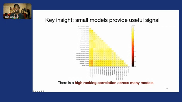
And we found that actually there’s a very high ranking correlation across many different models. So if we were to select the best examples from one model, it’s very likely that would be a good set of examples for us to label for another model. So we can actually exploit this by taking small, less accurate models and using them as inexpensive proxies during the data selection process.

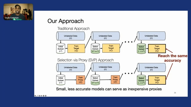
We call this approach “selection via proxy.” So the surprising thing is that even though these models are smaller and less accurate, they provide useful signals for selecting data. And once we take the final selected dataset and we train our kind of larger, more accurate model on it, we actually find that they reach the same accuracy.

This allows us to accelerate data selection and active learning by close to 42x. That’s a massive improvement, allowing us to scale to datasets that we couldn’t efficiently train on or work with before. So to quantify this and see if we actually picked useful examples, we evaluated our approach on a number of large-scale datasets.

Starting with CIFAR10, here the x-axis represents the amount of data that we’ve labeled so far—so our labeling budget. And then our y-axis is “Top-1 Test Error” for a model that we’re training. The dashed gray line represents the performance that we get if we train on the entire dataset. And then the black line represents what we’d get if we were just to take a random subset of that certain percentage of data.

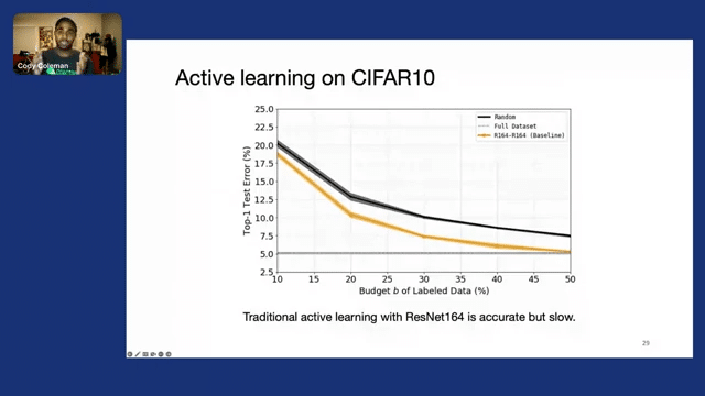
If we do traditional active learning with a very accurate model like ResNet164, we see that it’s accurate and we can actually get to basically the same level of accuracy with 50% of the data by doing this active learning technique, where it would take us all a hundred percent of the data to do that with random sampling. So we’re getting a 2x improvement in data efficiency. However, this process is really slow.

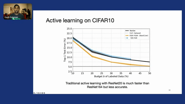
Alternatively, if we were to use a smaller model like ResNet20, which is much faster to train—about eight times faster to train–we can actually do this process relatively quickly. But ultimately, we can see by the dashed blue line that the final model’s performance isn’t that great—we have a much higher error than we did with ResNet164.

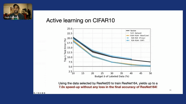
So what we ultimately want is to have the best of both worlds. And luckily we can actually do that by taking the data that was selected by ResNet20, and then training ResNet64, only at the end, once we’ve exhausted our labeling budget. We find that this yields a 7x speed up without any loss in the final accuracy of ResNet164, as shown by the overlapping solid blue and orange lines.

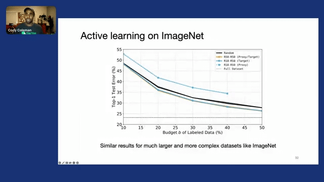
We performed the same experiment on many other datasets with other models. So on ImageNet, we see very similar results for this larger, more complex dataset. Here, we’re using ResNet18 to select data for a ResNet50 model.

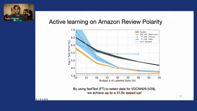
And then on Amazon reviews, with several million reviews, we actually take a very small, shallow model, fastText–which can be trained in a matter of minutes on the laptop–to select data for a much larger model, VDCNN29, which takes close to 16 hours to train on GPUs. And we find that we can actually speed up the process of data selection by close to 42x while allowing VDCNN29 to achieve effectively the same test error.

We’re not just limited to figuring out which data points to label in active learning. We can also use this process of selection via proxy to distill down large label datasets.

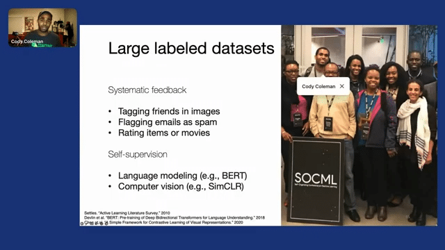
So where might we have these large label datasets? This comes up in practice if you have systematic feedback or feedback from users. So imagine you’re tagging friends and images on a social media website, you’re flagging emails as spam, or you’re rating items or movies on your favorite content-streaming platform. And when we think about these kinds of large self-supervised models—things in language modeling like BERT or GPT, or in computer vision like SimCLR and DINO—we effectively turn all of our unlabeled data into training data that we can use, which creates this massive dataset that would be awesome if we could distill down to some core-set.

And I don’t have time to dive deeply into the results, but we can apply the same idea of selection via proxy to this problem of core-set selection, where we effectively take our small proxy model that’s quick to train—we can train it on all of our label data—and then we can use that model to filter out unnecessary data points and only train our larger, more accurate model on that reduced subset.

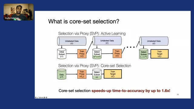
And we find that even for fairly small and balanced datasets like CIFAR-10, we can still achieve an end-to-end training time speed up of 1.6x without any loss in accuracy of the final model. And please see our work, our paper “Selection via Proxy” from ICLR 2020 for more details on core-set selection, as well as all of the other datasets and methods that we tried there.

Moving on to more recent work. “Similarity Search for Efficient Active and Learning Search of Rare Concepts” takes this idea of trying to really reduce the computational bottlenecks to another degree.

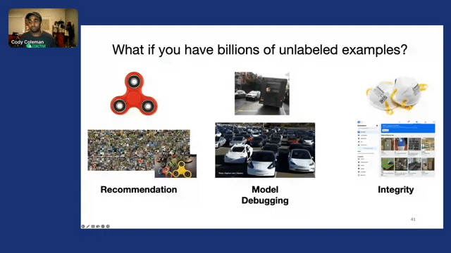
So let’s imagine that we’re at a really large-scale company with tremendous amounts, billions of unlabeled examples. So this might come up if we’re a social media site and we’re trying to do a recommendation. Imagine that something new happens that you want to identify. So for example, in 2015, fidget spinners were all the rage. Now you’re in luck because you have a lot of unlabeled or weakly labeled data, so there must be many more examples there for you to pull on to actually create a robust classifier. The problem is actually finding them. They only represent a very small percentage of your overall data. And this same type of problem where you have a very skewed data set and a tremendous amount of unlabeled data comes up over and over again.

For example, in working with folks in autonomous vehicles, they actually have this problem when they’re trying to debug a model for an autonomous vehicle. Imagine that you’re an autonomous vehicle company with a fleet of vehicles, and you notice that your car is getting stuck behind delivery trucks because it can’t tell a delivery truck from a normal truck.

What you would want to do in order to solve that problem is to actually go find data for delivery trucks so that you can build a classifier and plan around it so that you can move around delivery trucks. And this comes up all the time, so things like occluded stop signs, as well as debris on the road–all these edge cases only appear in a fraction of the overall data, which is like a needle in a haystack problem.

And finally, from an integrity standpoint, imagine that we’re a large e-commerce platform where we have a tremendous amount of different posts and items that are being sold. But if we go back to the beginning of the pandemic, there was a shortage of N95 masks, and it was socially unacceptable and illegal in some places to actually sell N95 masks because of a shortage of the supply. In that case, you really quickly wanna be able to create a robust classifier so that you can identify N95 masks and take down postings, so that you can disincentivize people from posting them and reserve the supply for the people that really need it.

So in all these cases, doing active learning as we laid out before will help us actually identify the best examples to improve our model out of this massive pool of unlabeled data that we have. But when we think about billions of unlabeled examples, now the bottleneck becomes just actually processing all of the unlabeled data, actually going through all of it to quantify its informativeness and label it.

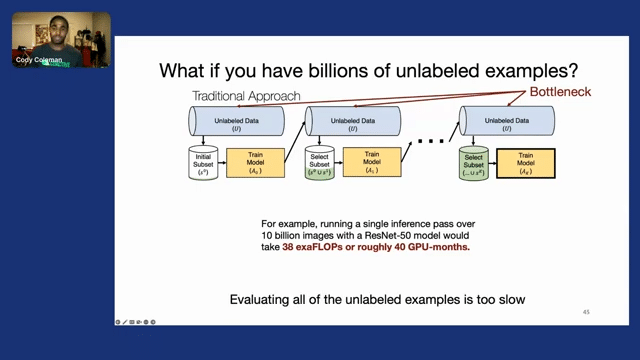
And many active learning strategies are linear in terms of the unlabeled data, and many others are actually quadratic, making it really hard to scale to these large datasets. So for example, even if you had to do a linear approach, simple uncertainty sampling, running a single inference pass over 10 billion images with a ResNet50 model would be about 40 exaFLOPs or roughly 40 GPU-months. This means that just evaluating all these unlabeled examples is effectively too slow and intractable for many users and use cases, especially when we want to do it multiple times in a process like active learning to be able to adapt to the data that we’re getting back.

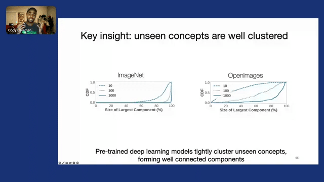
Now the key insight that we had in solving this is that we noticed that unseen concepts are actually well clustered by pre-trained deep learning models or foundation models. And effectively in the latent space, they form kind of tight clusters for these unseen concepts that are very well-connected components. So in these two plots, we actually calculated the largest connected component based on the K-nearest neighbor graph for different values of k and we plotted the CDF.

And what we can see is that both for ImageNet and OpenImages, the majority of classes actually form these very large connected components that have over 80% of the data, if you have a sufficiently large value of k. So what this means, if we visualize this, if we think about a simple example, when we think about the latent space, these data points actually have clusters together where your K-nearest neighbors for a single concept might be very close to one another in a connecting component, as shown in red.

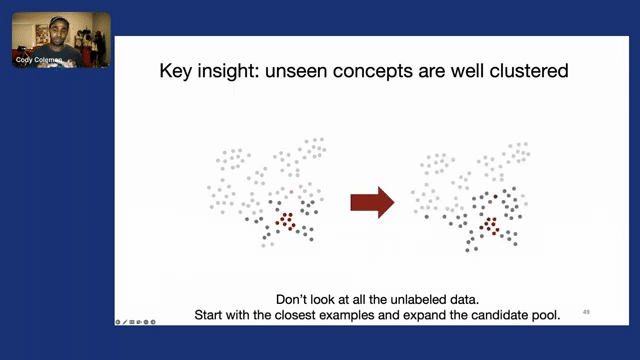
And what this means is that we actually don’t need to look at all of the unlabeled data. Most of the data for a single concept, if we’re thinking about N95 masks or delivery trucks or anything like that, actually only represents a very small fraction of this latent space. So we don’t actually need to look at all of the unlabeled data, and we can instead start with the closest examples to the seed set that we originally have, and then expand that candidate pool over time as we label more examples.

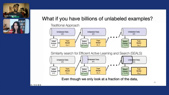
And this insight led to our approach similarity search for efficient active learning and search of rare concepts. And in this approach, we started off in the same way. So we have a large amount of unlabeled data, and we have some initial labeled subset that’s given to us, and we train a model on that initial subset. But instead of applying our selection strategy to all of the unlabeled data, we use similarity search to find the closest examples, and we only consider them.

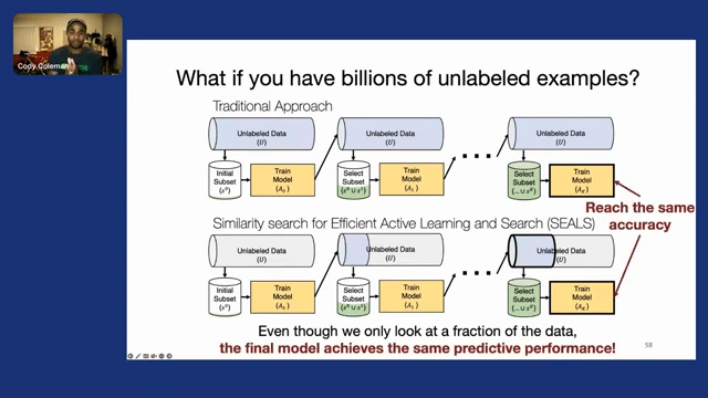
And then from that small candidate pool, we select the best examples within that neighborhood to label, and then we update our labeled set and we repeat this process. Then we take those newly labeled examples and we find their nearest neighbors to expand the candidate pool and the unlabeled data and repeat this process.

And then at the end, we’ve actually only looked at a very small fraction of the unlabeled data, but surprisingly, we find that the final model still achieves the same predictive performance. So this means that we only need to process a small fraction of the data, speeding up the process end-to-end, while getting the same accuracy.

To evaluate this and to see we actually focused on the right examples in the right part of the latent space, we evaluated this on a number of large-scale datasets. So here, the x-axis is the number of labels, the y-axis is our mean average precision for a subset of classes, and the gray dashed line represents the performance that we get with full supervision.

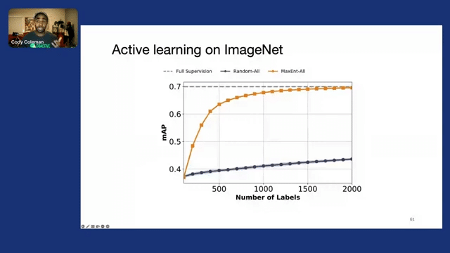
And then if we look at random sampling or passive learning, we see that with 2000 labels, we actually don’t get to a reasonably high accuracy. But if we were to do something like max entropy uncertainty sampling over all of the data, we can very quickly get close to full supervision with just a very small fraction of the data, A huge gap in comparison to random sampling, which dramatically improves the data efficiency and reduces the cost that we have for labeling as well as training.

However, this process is slow because again, we’re scanning over all of the data. But if we apply our SEALS method, we realize a very similar level of quality in terms of mean average precision, but we only end up considering less than 10% of the unlabeled data.

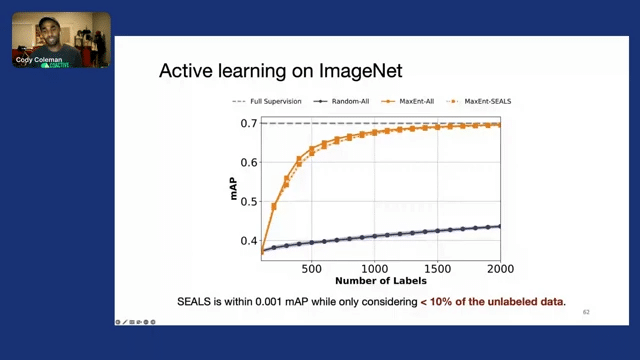
So this actually enables us to get a 5x speed up for a simple linear approach like uncertainty sampling, and up to a 50x speed up for larger or more complex methods like information density.

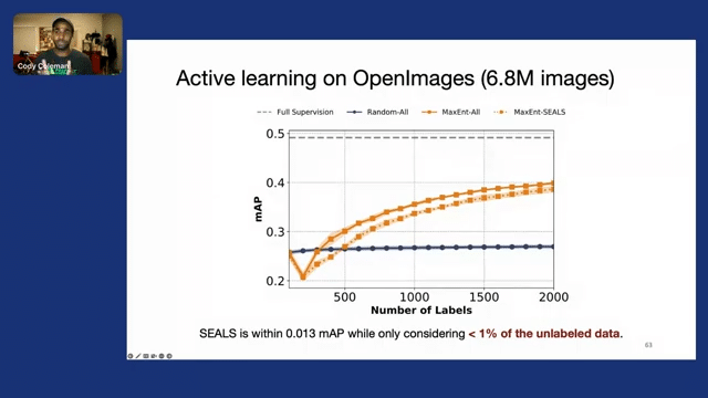
And as we increase the size of the dataset—OpenImages, at the time of this work, had 3.8 million examples that were available—we find that once again, SEALS achieves a very similar mean average precision, but now we actually only need to look at 1% of the unlabeled data. So now even a baseline approach, like max entropy, has a 50x speed up. And then once we get to more complex methods that scale quadratically or close to quadratically, we can get three orders of magnitude speedups in comparison to them.

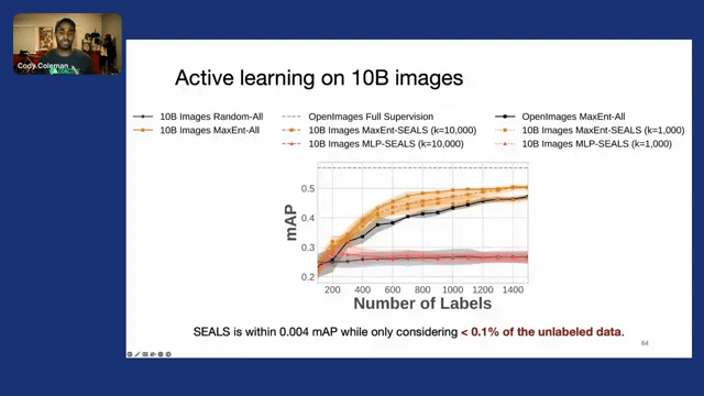
And finally, to really test this, to really put this at scale, we created a dataset of 10 billion images from a social media platform from a large internet company, and we applied SEALS to that. And we found that once again, that the SEALS method achieves a very similar mean average precision to the baseline approach that scans over all of the data, but we only need to look at less than 0.1% of the unlabeled data.

What this means is, in practice when we ran this method, we needed a cluster of machines in order to do a single pass. But with SEALS, we could actually do it on a single data machine, on a single personal computer.

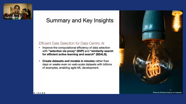
This is amazing because we can improve the computational efficiency of data selection with methods like selection via proxy and SEALS. And that allows us to create datasets and models in minutes rather than days or weeks, even on web-scale datasets with billions of examples, enabling agile ML development and allowing humans and machines to work together more efficiently and quickly.

Question and answer session

Aarti Bagul: Amazing. Thank you so much Cody for that excellent presentation. I’m seeing a lot of appreciation in the chat, and then we have a bunch of Q&As also popping up. I’ll ask you a couple of questions. So the first one that popped up is, “in the similarity search, how do you decide on your candidate pool?”

Cody Coleman: Yeah, that’s a great question. So in the similarity search, what we’re doing is we’re taking that labeled set that we have after each round, we’re finding the nearest neighbors of those labeled data points in the unlabeled data, and we’re effectively—to keep the computation of the similarity search down—using an approximate K-nearest neighbors algorithm, which can scale to billions of examples with sub-second latency.

AB: Got it. Thank you. I guess, related to the similarity search, Daniel asked, “will similarity search-based sampling strategy make it even more difficult to properly learn rare classes in the dataset?”

CC: Yeah, this is a great question. So what we found going back to this kind of key insight is that rare concepts we find are actually fairly well clustered in the data as we get better and better representations. When we think about these foundation models, when we think about search in general, they’re meant to create these representations that kind of create a very nice latent structure, which makes things very easy downstream. This is why when we think about papers like GPT2, where they these large language models are effectively few-shot learners, that’s partially because of the fact that we can actually create the examples in that space, which makes it very easy to separate and to classify. But of course there are edge cases where there are ambiguous things. In OpenImages, for example, there’s a class called “electric blue.” Electric blue can appear in many different things, and that can actually be a difficult example because it’s spread over the entire space. But for things that are very visually obvious that the representation picks up well, they’re actually very well clustered.

AB: Got it. Thank you. People are very excited about the clustering approach, so another question is, “the K-means algorithm is a partitioning, not a clustering technique. Have you tried other clustering approaches like bonafide clustering approaches such as DBSCAN on such large datasets? Thank you.” That’s the question. So have you tried other clustering approaches other than K-means, and how does that impact this entire process?

CC: Oh, yes. That’s a great question. We’re not exactly using the K-means algorithm, we’re using more of a K-nearest neighbors approximate algorithm, just to be able to get this kind of very quick look-up for a single data point to find its nearest neighbors. We actually don’t want to cluster everything if we don’t have to. And just by being able to actually find the nearest neighbors, which is a slightly different problem than true clustering, that’s where we get our benefit because we can effectively explore this K-nearest neighbors graph, going one edge at a time, almost in a traditional search algorithm, or things like that. We use the model’s uncertainty to direct that. It’s a slightly different setup than maybe a more traditional clustering algorithm. Our approach is really the speed and the fact that similarity search is very well optimized at a large scale. Since it’s a backbone application, we can actually exploit that to make this processing really fast.

AB: Makes sense. It’s optimized for the problem that you’re trying to tackle, which is trying to work with this really large unlabeled dataset. Around that, I guess people are curious about the robustness and dealing with rare classes. So we have questions like “have you checked this against out-of-domain distribution, generalization, or robustness dataset or metrics?” We’re just curious about that trade-off here when you are sampling the nearest neighbors. I know you touched on this previously but any thoughts around if these models are still as robust or do they still generalize well, as part of your evaluation process?

CC: Yeah, that’s a great question. If the data is out of distribution for the embedding model that you use, or the algorithm, the representation that you’re using for similarity search, then you can run into problems. So I believe in the paper we had one case of this with Goodreads, where we use a traditional Sentence-BERT model that’s trained in a traditional way. And so it’s going to basically classify content or it’s going to cluster content together that have similar themes, in a sense. But then the task that we wanted to do with Goodreads was to detect if a review was a spoiler or not. So it’s actually a very different distribution of data and a different problem than what the original embedding model and similarity search was trained on. And in that case, it can be a little bit harder to have a good distribution and results, so the robustness is a little bit more difficult there. But increasingly, as we get to better representations and things like that. and we can quickly change for different tasks, you can imagine improving that even for these kinds of different distributions. But that is definitely a problem if your similarity search engine was trained on a very different task than the classifications that you’re trying to do.

AB: Makes sense. We do have a lot more questions popping in, so if people have more questions—and there are a bunch—how can they best contact you to ask you more questions after this?

CC: Yeah, great question. Yeah, so feel free to email me at cody@coactive.ai. That’s probably the best way to get in touch with me. So thank you for all of the questions. This was an awesome session.

Build and evaluate LLMs faster than ever with Snorkel + AWS

Snorkel AI and AWS have launched an accelerator program for Amazon SageMaker customers designed to deliver private fine-tuned generative AI models along with co-developed benchmarks that evaluate model performance against an organization’s unique goals and objectives.  Learn more and apply here or book a meeting at AWS re:Invent 2024.